One-Way ANOVA F-Test
Simplest ANOVA
- are the means of several groups equal?
- it’s a Statistical Test
- And it generalizes the t-tests
It’s an $F$-Test
- We assume that we have Normal Distribution
- and the resulting value follows the $F$-Distribution
It’s a parametric test of Variance:
- it’s parametric because it’s based on Normality hypothesis
Comparing Means
Comparing means of several groups
- We can compare means of two groups using Two-Sample $t$-test
- But sometimes we want to compare means across many groups
First idea: do Pairwise comparison
- but we may find the difference just by chance, even when there’s no difference - because there’ll be too many comparisons
- need to do some correction
Test Of Independence
One-Way ANOVA can be used to analyze the relationships between two variables
- numerical and categorical
- we group the numerical one by associated categories
- and find the means of each category
- then we test if the means are the same
- if yes - these two variables are independent
Post-ANOVA Comparison
suppose we reject $H_0$
- we may wonder, which groups are different?
- to find out, can use the following tests:
- Pairwise $t$-test note that in this case we need to reduce Family-Wise Error Rate e.g. with Bonferroni Correction
- Tukey HSD Test
The One-Way ANOVA Test
ANOVA: compare many means in a single hypothesis
- are the means of several groups equal?
- so it generalizes the $t$-test to more than two groups
- used in Bivariate Analysis to test if a numerical and categorical variables are independent
ANOVA:
- assessing the variability of the group mean relative to variability among individual observations
- the questions answered: “is the variability on the sample means so large that it seems unlikely to be entirely due to chance?”
General Idea:
- simultaneously consider many groups
- evaluate if the sample means differ more than we’d expect from natural variation
Assumptions
- observations are independent
- data within each group is distributed normally
- variability across the groups is approximately equal
ANOVA Test
- $H_0: \mu_1 = \mu_2 = … = \mu_k$
- $H_A:$ at least one $\mu_i$ is different from the rest
Estimating variability:
- this variability is called MSG: mean square between groups
-
$\text{df}_G = k - 1$ for $k$ groups
- let $\bar{x}$ be the sample mean across all groups
- $\text{MSG} = \cfrac{1}{\text{df}G} \cdot \text{SSG} = \cfrac{1}{k - 1} \sum{i=1}^k n_i (\bar{x}_i - \bar{x})^2$
- $\text{SSG}$ - sum of squares between groups
- $n_i$ - sample size of group $i$
this gives us a base point, and we compare it with $\text{MSE}$:
$\text{MSE}$: mean square error (pooled variance estimate)
- $\text{df}_E = n - k$
- $\text{SST} = \sum_{i=1}^n (x_i - \bar{x})^2$
- sum of squares total
-
this is calculated over all observations in the data set
- $\text{SSE} = \text{SST} - \text{SSG} = (n_1 - 1) \cdot s^2_1 + (n_2 - 1) \cdot s^2_2 + … + (n_k - 1) \cdot s^2_k$
- $s^2_i$ - sample variance of residuals in the group sum of squared error standardized form of $\text{SSE}$: $\text{MSE} = 1 / \text{df}_E \text{SSE}$
if $H_0$ is true then differences are due to chance and MSG and MSE should be approximately equal
Then we can calculate the test statistics $F = \cfrac{\text{MSG}}{\text{MSE}}$
- $\text{MSG}$ = between the group variability
- $\text{MSE}$ = withing the group variability
$F$ is a $F$ statistics that follows $F$-distribution it has 2 associated parameters: $\text{df}_1$ and $\text{df}_2 $ for ANOVA it’s $\text{df}_G$ and $\text{df}_E$
the larger $\text{MSG}$ relative to $\text{MSE}$, the larger $F$ is, and the stronger evidence against $H_0$
We use upper tail to compute the $p$-value
Test (From Data Mining (UFRT))
Given
- $X$ with $k$ possible values $x_1, …, x_k$ - categorical variable (e.g. Job)
- and $Y$ - continuous variable (e.g. Age)
Let
- $\mu = \text{mean}(Y)$: Mean value of $Y$
- $\mu_k$: mean value of $Y$ for tuples such that $X = x_k$
- $N_k$ : number of records such that that $X = x_k$
- $N = \sum_k N_k$ : total number of records
Define:
- Interclass Variance: $\text{Inter} = \cfrac{1}{K-1} \cdot \sum_k N_k \cdot (\mu_k - \mu)^2$
- total variance
- Intraclass Variance: $\text{Intra} = \cfrac{1}{N-K} \cdot \sum_k \sum_{j : X = x_k} ( y_j - \mu_k )^2$
- variance inside each group
Test
- to evaluate the correlation between $X$ and $Y$ calculate $F = \cfrac{\text{Inter}}{\text{Intra}}$
- the null hypothesis $H_0$: all means $\mu_k$ are equal (i.e. assume independence),
- under $H_0$ $F$-ratio follows $F_{K-1,N-K}$: $F$-distribution with $K-1,N-K$ degrees of freedom
- if independent, all the means should be the same for all classes and $F$ should be 0
Examples
Example 1: Baseball
Batting Performance
we have 4 categories of baseball players:
- outfielders: $\text{OF}$
- infielders: $\text{IF}$
- jilter: $\text{DH}$
- catcher: $\text{C}$
Is there any difference in performance? (using on-base percentage OBP to measure it)
Test:
- $H_0: \mu_\text{OF} = \mu_\text{IF} = \mu_\text{DH} = \mu_\text{C}$
- $H_A$: at least one is different
we approximate each $\mu$ by $\bar{x}$
| OF | IF | DH | C | + Summary statistics (source: table 5.27, OpenIntro) | Sample size ($n_i$) | 120 | 154 | 14 | 39 | Sample mean ($\bar{x}_i$) | 0.334 | 0.332 | 0.348 | 0.323 | Sample SD ($s_i$) | 0.029 | 0.037 | 0.036 | 0.045 |
 (source: fig 5.28, OpenIntro)
We see that DH and C look really different. Why don’t we just check if $\mu_\text{DH} = \mu_\text{C}$?
- the primary issue: we’re inspecting the data before doing the check
- this is called Data Snooping (or Data Fishing)
- naturally we’d pick up the groups with largest differences and run the formal test
- but it would lead to Type I Errors
- it’s also called Prosecutor’s Fallacy
Calculate:
- $\text{MSG} = 0.00252$
- $\text{MSE} = 0.00121$
- $k = 4$ groups, $\text{df_G} = 4 - 1 = 3$
- $n = n_1 + n_2 + n_3 + n_4 = 327$, $\text{df}_E = n - k = 323$
- $F = \cfrac{MSG}{MSE} = \cfrac{0.00252}{0.00121} \approx 1.994$
P-value
- $p$-value is 0.115 > 0.05
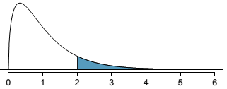
- so we fail to reject $H_0$ at the significance level $\alpha=0.05$
Example 2: Statistics Class
We have high demand for a course, so run it several times in one semester
- e.g. it’s run 3 times: scores of each run are sets $A, B, C$
- are these significant differences?
Test:
- $H_0: \mu_A = \mu_B = \mu_C$
- $H_A:$ scores may vary on average
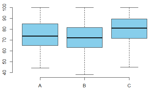
| Group | $n$ | Min. | Mean | Max. | Std | $A$ | 58 | 44 | 75.10 | 100 | 13.86867 | $B$ | 55 | 38 | 71.96 | 100 | 13.77056 | $C$ | 51 | 45 | 78.94 | 100 | 13.12008 |
We run ANOVA tests and obtain the following summary table:
| Df | Sum Sq | Mean Sq | $F$ value | $Pr(>F)$ | lecture | 2 | 1290.11 | 645.06 | 3.48 | 0.0330 | Residuals | 161 | 29810.13 | 185.16 |
The $p$-value is greater than $\alpha=0.05$, so we reject $H_0$
library(openintro)
data(classData)

by(classData$m1, classData$lecture, summary)
by(classData$m1, classData$lecture, sd)
by(classData$m1, classData$lecture, length)


boxplot(classData$m1 ~ classData$lecture, col='skyblue', axes=F)
axis(side=2)
axis(side=1, at=1:3, labels=c('A', 'B', 'C'))


oneway.test(classData$m1 ~ classData$lecture, var.equal=T)
1. or
aov1 = aov(classData$m1 ~ classData$lecture)
summary(aov1)
Post-ANOVA processing: use $t$-test to pairwise compare $A,B,C$
- With Bonferroni Correction, $\alpha^* = \alpha / 3 = 0.05 / 3 = 0.017$
- $A$ vs $B$: $p$-value is 0.228, don’t reject
- $A$ vs $C$: $p$-value is 0.148, don’t reject
- $B$ vs $C$: $p$-value is 0.01, reject
In R:
pairwise.t.test(classData$m1, classData$lecture,
                alternative='two.sided', p.adjust.method='bonferroni')
Or
TukeyHSD(aov1)
Example 3: Donuts
Example from link
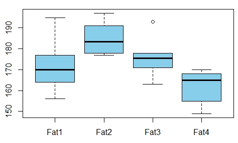
- study of donuts: the relationship between the amount of absorbed fat vs the type of fat
- is there any relationship?
The data:
| Fat1 | Fat2 | Fat3 | Fat4 | 164 | 178 | 175 | 155 || 172 | 191 | 193 | 166 || 168 | 197 | 178 | 149 || 177 | 182 | 171 | 164 || 156 | 185 | 163 | 170 || 195 | 177 | 176 | 168 |
We run ANOVA analysis and get the following:
- $F = 5.4063$,
- num $\text{df} = 3$, denom $\text{df} = 20$,
- $p\text{-value} = 0.006876$
file = 'http://courses.statistics.com/software/data/donuts.txt'
donuts = read.table(file, header=T)
donuts = stack(donuts)
donuts

boxplot(donuts$values ~ donuts$ind)
oneway.test(donuts$values ~ donuts$ind, var.equal=TRUE)
1. p\text{-value} is small, we reject the hypothesis of equal absorption.
Same, done in steps:
groups = 4
1. total variance
df.g = groups - 1
tot.mean = mean(donuts$values)

group.mean = tapply(donuts$values, donuts$ind, mean)
n = tapply(donuts$values, donuts$ind, length)

inter = sum(n * (group.mean - tot.mean) ^ 2) / df.g

1. variance inside each group
df.e = length(donuts$values) - groups
intra.1 = tapply(donuts$values, donuts$ind, FUN=function(data) {
  m = mean(data)
  sum( (data - m)^ 2)
})
intra = sum(intra.1) / df.e

F.stat = inter/intra
F.stat

p = 1 - pf(F.stat, df1=df.g, df2=df.e)
p
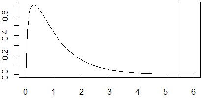
x = seq(0, 6, 0.05)
y = df(x, df1=df.g, df2=df.e)
plot(x, y, type='l')

abline(v=F.stat)
Links
- Good example: http://en.wikipedia.org/wiki/F_test#One-way_ANOVA_example
Sources
- OpenIntro Statistics (book)
- Data Mining (UFRT)
- http://en.wikipedia.org/wiki/Analysis_of_variance