Residual Analysis

statistics

Residuals

'’Residuals’’ is the difference between actual values and predicted values

$i$th residual is:

Mean of $e$:

$\bar{e} = \bar{y} - b_0 - b_1 \bar{x} = \bar{y} - (\bar{y} - b_1 \bar{x}) - b_1 \bar{x} = 0$

What about $\text{Var}(e)$?

$e_i = y_i - b_0 - b_1 x_i = y_i - (\bar{y} - b_1 \bar{x}) - b_1 x_i = (y_i - \bar{y}) - b_i (x_i - \bar{x}) = (y_i - \bar{y}) - R \cfrac{s_y}{s_x}(x_i - \bar{x})$
so,

$(e_i - \bar{e})^2 = (y_i - \bar{y})^2 + (R \cfrac{s_y}{s_x})^2 (x_i - \bar{x})^2 - 2 (\bar{y} - b_1 \bar{x}) \cdot R \cfrac{s_y}{s_x}(x_i - \bar{x})$
$\text{Var}(e) = \cfrac{1}{n - 1} \sum (e_i - \bar{e})^2 = s_y^2 + (R \cfrac{s_y}{s_x})^2 s_x^2 - 2R \cfrac{s_y}{s_x} \cfrac{1}{n - 1} \sum (x_0 - \bar{x})(y_i - \bar{y}) = $ (note the orrelation coefficient again| ) |- $= s_y^2 + R^2 s_y^2 - 2R\cfrac{s_y}{s_x} s_x s_y R = s_y^2 + R^2 s_y^2 - 2R^2 s_y^2 = s_y^2 (1 - R^2)$ |

So

$\text{Var}(e) = \text{Var}(y)(1 - R^2)$

The regression multiplies the variance of $y$ by $(1 - R^2)$

Or, the regression line ‘‘removes’’ (or ‘‘reduces’’) a fraction of $R^2$ of the variance of $y$
Or we say it “explains a fraction of $R^2$ of the variation”

$R^2$ is called ‘‘coefficient of determination’’ - and says what fraction of $\text{Var}(Y)$ has been explained by the linear relationship

Examples:

$R^2 = 0$: the linear relationship explains nothing (so no linear relationship between $X$ and $Y$)
$R^2 = 1$: the linear relationship explains everything - no left-overs, no uncertainty
$R^2 = 0.0186$: only 1.86% of variation was explained by the linear model - so there hardly is a linear relation. The rest of the variance (98%) is due to something else

Let’s take a look at the example again:

<img src=”” />
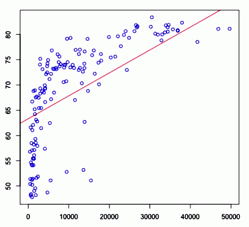$R^2$ = 0.4033
so it means quite a bit of variance there is explained by linear model
but still it doesn’t explain everything - indeed the real data doesn’t seem to have linear relationship

Are there any other kinds of relationships between $X$ and $Y$, not captured by regression?

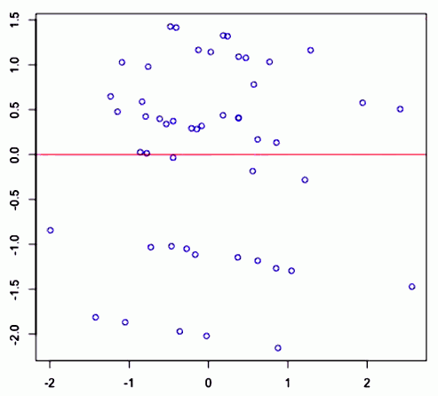This is a good case because after taking out linear relationship there’s no particular pattern in residuals: only independent errors are left
So overall there’s no particular trend and that means that the regression really tells us something about the relationships between $X$ and $Y$

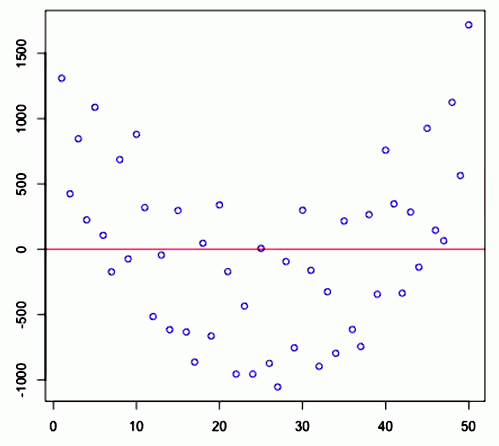And the same here

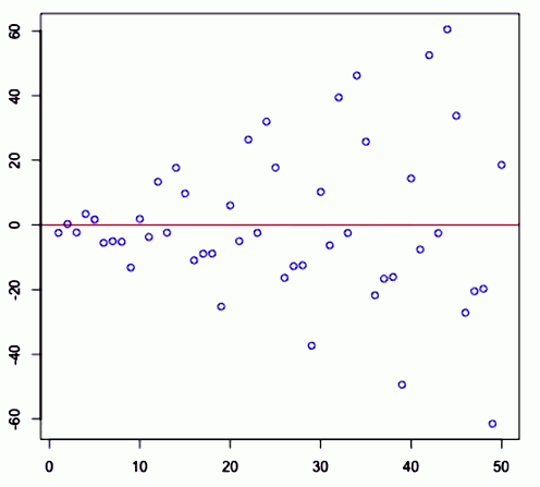In both cases the linear relationship doesn’t describe the whole story and we see there are apparent patterns in the residuals in both cases

To improve the situation we could try to transform the variables before applying regression.
Most common transformation is logarithmic

So we have the following:

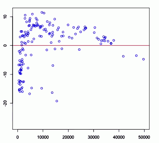Recall that in this case $R^2 = 0.40$

If we calculate $\log_{10} x$ what we get is

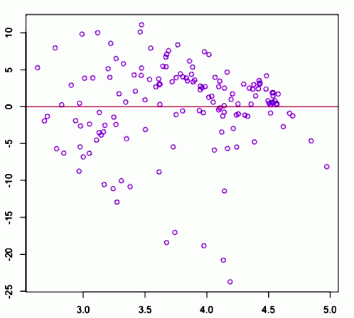Now we’re able to fit a better regression line and in this case $R^2 = 0.6576$

Here we interpret a slope of 14.93 as

✏️ Edit on GitHub