Contents
Confidence Intervals for Means
We want to build a Confidence Interval for a Point Estimate of the population mean
Problem
- let $\mu$ be the true mean parameter
- $X_1, ..., X_n$ our sample of size $n$
- $\bar{X}$ - the average value for the sample $\bar{X} = \cfrac{1}{n} \sum_{i=1}^n X_i$
- we want to estimate $\mu$ using $\bar{X}$ and a Confidence Interval around it
Normal Model
With sufficiently large sample and no violations of the assumptions, we can use Normal Distribution to model the Sampling Distribution of mean
- note that it's better to use the $t$ statistics described below
Normal Approximation
Normal approximation is crucial for this - because we use Normal Distribution to find percentiles
Assumptions
- sample observations are independent
- the distribution is not strongly skewed and there are few outliers
- sample size is sufficiently large (e.g. $\geqslant 30$)
- the larger the sample, the more tolerant we can be to the skews (thanks to the C.L.T)
- sampling distribution is symmetric, unimodal, no outliers - approximately normal
If these conditions are met, can use Normal Model to find the confidence intervals
Example
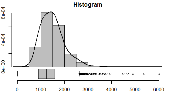
We have this data set that contains data about the whole population
Suppose we take 10k samples
- and for each sample we calculate the mean
- and then draw the histogram of this data - thus we'll get the sampling distribution
-
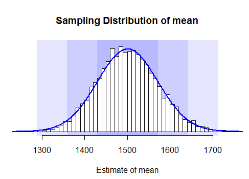
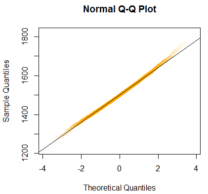
- we see that it's normal, but can also try to draw the Normal Probability Plot to see that it's indeed the case
-
load(url('http://s3.amazonaws.com/assets.datacamp.com/course/dasi/ames.RData'))
population = ames$Gr.Liv.Area

oldpar = par(no.readonly=TRUE)

# fig=c(x1, x2, y1, y2)
par(fig=c(0, 1, 0, 1))
par(mar=c(6, 2, 2, 1))
h = hist(population, col='grey', probability=T, axes=F, xlab='', main='Histogram')
dens = density(population, adjust=2)
lines(dens, col="black", lwd=2)

axis(side=1, pos=c(-max(h$density)/4,0))
axis(side=2)

par(fig=c(0, 1, 0.16, 0.41), new=TRUE)
par(mar=c(0, 2, 0, 1))
boxplot(population, horizontal=TRUE, axes=F, col='grey')

par(oldpar)

set.seed(1237)
n = 50
samp.mean = replicate(10000, mean(sample(population, n)))

plot(x=NA, y=NA, xlim=c(1250, 1750), ylim=c(0, 0.006), axes=F,
     xlab='Estimate of mean', ylab='Frequency',
     main='Sampling Distribution of mean')

m = mean(samp.mean)
s = sd(samp.mean)

par(xpd=FALSE)

rect(xleft=m-3*s, xright=m+3*s, ybottom=-1, ytop=1,
     border=NA, col=adjustcolor('blue', 0.1))
rect(xleft=m-2*s, xright=m+2*s, ybottom=-1, ytop=1,
     border=NA, col=adjustcolor('blue', 0.1))
rect(xleft=m-s, xright=m+s, ybottom=-1, ytop=1,
     border=NA, col=adjustcolor('blue', 0.1))

hist(samp.mean, probability=T, add=T, breaks=50, col='white')
axis(side = 1)

dens = dnorm(1200:1800, mean=m, sd=s)
lines(1200:1800, dens, col="blue", lwd=2)


qqnorm(samp.mean, col=adjustcolor('orange', 0.1))
qqline(samp.mean)
In this case all the assumptions hold - can use the Normal Approximation to calculate the confidence intervals
Model
- $E[\bar{X}] = \mu$, it's an unbiased estimate of mean
- Standard Error: $\text{var}(\bar{X}) = \cfrac{\sigma^2}{n}$
- by C.L.T. have $\bar{X} \approx N\left(\mu, \cfrac{\sigma^2}{n}\right)$
- therefore
- $\cfrac{\bar{X} - \mu}{\sqrt{\sigma^2 / n}} \approx N(0, 1)$
So the 95% CI with $z$-score is:
- $\left[ \bar{X} - 1.96 \sqrt{\sigma^2 / n}; \bar{X} + 1.96 \sqrt{\sigma^2 / n} \right]$
Estimating $\sigma$
To compute a CI we need to know $\sigma^2$, but it's a parameter - we need to estimate it
- We know that
- $\text{Var}(X) = \cfrac{1}{n - 1} \sum (x_i - \bar{X})^2 $
- $s = \text{sd}(X) = \sqrt{\text{Var}(X)}$
- $\sigma^2$ is unknown. Can we substitute it by $s^2$?
- $s^2$ is unbiased estimate of $\sigma^2$
- $E[s^2] = \sigma^2$ (this is the reason for $n - 1$ instead of $n$)
- so yes, we can, but it's better to use the $t$-distribution (described below) instead and use $s^2$
Using $t$ Statistic
To use normal approximation we need a sufficiently large sample
- what if we don't have it?
- use $t$-statistics that follows $t$-distribution
- note that with high degrees of freedom $t$-distribution very closely resembles $N(0,1)$
$t$-distribution
$t$-distribution
- We say that value follows $t$-distribution with $n - 1$ degrees of freedom
- This distribution is similar to normal, but not quite: it's little wider and allows for more uncertainty
Use the $t$- distribution rather than the normal distribution when
- the variance is not known and
- has to be estimated from sample data.
Shape of $t$ vs Normal:
- When the sample size is large, e.g. $\geqslant$ 100, the $t$ is very similar to $N(0,1)$
- on smaller sizes, $t$ is leptokurtic - it has relatively more scores in its tails than the normal distribution
- $\Rightarrow$ you have to extend farther from the mean to span a given proportion of the area.
- for $N(0,1)$ 95% of data is within 1.96 $\sigma$ from the mean
- for $t$, if you a sample size is only 5, 95% of the area is within 2.78 std from the mean
- $\Rightarrow$ the SE of the mean would be multiplied by 2.78 rather than 1.96.
$t$-Statistic Confidence Intervals
Thus
- we replace $\sigma^2 = s^2$ and
- use the $t$-distribution with $n-1$ degrees of freedom
- i.e. replace $z$-score with $z = t_{n - 1}$
95% CI becomes
- $\left[\bar{X} - t \cdot \sqrt{s^2 / 2}; \bar{X} + t \cdot \sqrt{s^2 / 2}\right]$
- we we have $n = 400$ (therefore $df=399$), $t \approx 1.969$
R-code
In R:
n = 60
xbar = mean(d)
v = var(d)
t = qt(0.025, df=n-1, lower.tail=F)
ME = t * sqrt(v / n)
xbar + c(-ME, ME)
or:
t.test(d, conf.int=0.95)$confint
The last chuck actually uses $t$-test and returns its confidence interval
Examples
Example1:
- The mean for 51 observations was 20
- The sample variance was 5
- Calculate the 99% CI for the mean
xbar = 20
v = 5
t = qt(0.005, df=50, lower.tail=F)
ME = t * sqrt(v / 50)
xbar + c(-ME, ME)
// [19.16, 20.84]
Links
Normal-distr based
- http://www.stat.wmich.edu/s160/book/node46.html
- http://onlinestatbook.com/2/estimation/mean.html
- http://stattrek.com/estimation/confidence-interval-mean.aspx
t-based CI for mean