ML Wiki

Regression

How to understand the linear relationship between data?

• dependent (response) variable - $Y$
• independent (explanatory) variable or predictor - $X$

To what extent $X$ can help us to predict $Y$?

Regression Line

The line has the followoing form:

• $y = b_0 + b_1 \cdot x$
• $b_0$ - intercept
• $b_1$ - slope

Suppose we have $n$ observations

• for $i$th observation we have $y_i = b_0 + b_1 x_i$
• and difference $y_i - b_0 - b_1 x_i$ is called residual
• We'd like to make these differences for all $i$ as small as possible

Method of Least Squares

Main Article: Method of Least Squares

To find the slope and the intercept parameters we may use the method of least squares

Interpretation

• Suppose we have $b_0 = -23.3, b_1 = 0.41$
• It means that

When $X$ increases by 1, $Y$ increases by 0.41

• $b_0$ value the regression would give if $X = 0$

or how much we have to shift the line

Symmetry

Regression is not symmetric:

regressing $X$ over $Y$ is not the same as regressing $Y$ over $X$

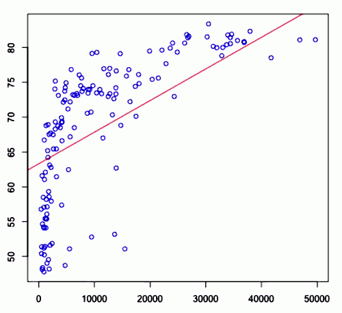
Example

This is an example of best linear fit:

Correlation

For intercept we have:

• $b_0 = \cfrac{1}{n} (\sum y_i - b_1 \sum x_i) = \bar{y} - b_1 \bar{x}$

So the regression line takes the following form

• $b_0 + b_1 x_i = (\bar{y} - b_1 \bar{x}) + b_1 x_i = \bar{y} + b_1 (x_i - \bar{x})$

This means:

• we start from mean of $y$
• and shift by how far we're from $\bar{x}$ multiplied by slope
• $(\bar{x}, \bar{y})$ is always on the line!

Let's manipulate it a bit the formula for the slope coefficient to get better understanding of what's going on

• $b_1 = \cfrac{n \sum x_i y_i - \sum x_i \sum y_i }{n \sum x_i^2 - (\sum x_i)^2} $ (divide top and bottom by $1/n^2$)
• $ = \cfrac{\frac{1}{n} \sum x_i y_i - \frac{1}{n} \sum x_i \cdot \frac{1}{n} \sum y_i}{\frac{1}{n} \sum x_i^2 - (\frac{1}{n} \sum x_i )^2 } $
• $= \cfrac{\frac{1}{n} \sum x_i y_i - \bar{x} \bar{y}}{\frac{1}{n} \sum x_i^2 - \bar{x}^2 } $
• $ = \cfrac{\frac{1}{n} (x_i - \bar{x})(y_i - \bar{y}) }{\frac{1}{n} \sum (x_i - \bar{x})^2 }$ (let's multiply top and bottom on $\sqrt{\sum (y_i - \bar{y}) }$)
• $ = \cfrac{(x_i - \bar{x})(y_i - \bar{y}) \cdot \sqrt{\sum (y_i - \bar{y})^2 } }{ \sqrt{\sum (x_i - \bar{x})^2 } \cdot \sqrt{\sum (x_i - \bar{x})^2 } \cdot \sqrt{\sum (y_i - \bar{y})^2 }} = R \cfrac{s_y}{s_x}$

So we get

$b_1 = R \cfrac{s_y}{s_x}$

where

• $s_x = \sqrt{\cfrac{1}{n - 1} \sum (x_i - \bar{x}) }$ and
• $s_y = \sqrt{\cfrac{1}{n - 1} \sum (y_i - \bar{y}) }$
• $R = \cfrac{\sum (x_i - \bar{x})(y_i - \bar{y})}{\sqrt{\sum (x_i - \bar{x})^2 \sum (y_i - \bar{y})^2 }}$ is the correlation coefficient

Residuals

Residuals is the difference between actual values and predicted values

$i$th residual is:

• $e_i = y_i - (b_0 + b_1 x_i) = y_i - b_0 - b_1 x_1 $

Residual Analysis

Main Article: Residual Analysis

Residual Analysis - is a powerful mechanism for estimating how good a regression is

• It gives us $R^2$, called Coefficient of Determination, which is a measure of how much variance in the data was explained by our regression model

Regression Inference

How much uncertainty is it there? Can we apply

• Confidence Intervals?
• Hypothesis testing?

We have a formula for slope $b_1$ and, let $\beta_1$ be the true value of slope

• How close $b_1$ to $\beta_1$?

There's the following fact:

• $\cfrac{b_1 - \beta_1}{\text{SE}(b_1)} \sim t_{n - 2}$
• where $\text{SE}$ is standard error
• we loose one degree because we don't know the slope and the other because of the intercept

And we calculate the standard error as

• $\text{SE}(b_1) = \cfrac{\sqrt{\sum e_i^2 }}{\sqrt{(n - 2) \sum (x_i - \bar{x})^2 } }$
• recall that $e_i = y_i - (b_0 + b_1 x_i)$

Confidence Intervals

So a $(1 - \alpha)$ CI for $\beta_1$ is

$b_1 \pm T_{\alpha/2, n-2} \cdot \text{SE}(b_1)$

Example

• $Y$ = age difference
• $X$ = bmi
• $n = 400$
• $b_1 = 0.41$
• $\sum e_i^2 = 78132$
• $\sum(x_i - \bar{x}) = 8992$

We're interested to calculate 95% CI:

• $0.41 \pm 1.97 \cdot \cfrac{\sqrt{78131}}{\sqrt{398 \cdot 8992}} = 0.41 \pm 0.29 = [0.12, 0.70]$

Hypothesis Testing

We may want to ask if there is any linear relationship.

So the following test gives an answer:

• $H_0: \beta_1 = 0, H_A: \beta_1 \neq 1$

For the example above we have

• $\cfrac{b_1 - \beta_1}{\text{SE}(b_1)} \sim t_{n - 2}$
• $b_1= 0.41, \text{SE}(b_1) = 0.148$

$p$-value (under $H_0$)

• $P( | b_1 - \beta_1 | \geqslant 0.41 ) = $
• $P \left( \left| \cfrac{b_1 - \beta_1}{\text{SE}(b_1)} \right| \geqslant \cfrac{0.41}{\text{SE}(b_1)} \right) \approx$
• $P( | t_{398} | \geqslant 2.77 ) \approx 0.0059$

Quite small, so we reject the $H_0$ and conclude that $\beta_1 \neq 0$, i.e. there is some linear relationship.

Limitations

• linear! - fails to predict other kinds of relationships (quadratic etc)
• not robust to outliers (just one outlier can change the regression line rather significantly)

Gradient Descent

Another way of finding the slope and intercept parameters is Gradient Descent Algorithm,

• which, usually, gives approximate solution,
• but works faster for Multivariate Linear Regressions

Multivariate Linear Regression

Main Article: Multivariate Linear Regression

We can use the regression to fit a linear model for several variables.

In R

# lm - linear model 
lm1 = lm(diff ~ bmi)

plot(diff ~ bmi)
abline(lm1)

# summary of regression
summary(lm1)

# the residual difference for each observation
lm1$residuals 

Logarithmic transformation

lm1 = lm(diff ~ log10(bmi))

Sources

• Statistics: Making Sense of Data (coursera)