Chi-Squared Test of Independence

Chi-Squared Test of Independence

This is one of $\chi^2$ tests

• one-way table tests - for testing Frequency Tables, Chi-Squared Goodness of Fit Test
• two-way table tests - for testing Contingency Tables, this one

$\chi^2$ Test of Independence

This is a Statistical Test to say if two attributes are dependent or not

• this is used only for descriptive attributes

Setup

• sample of size $N$
• two categorical variables $A$ with $n$ modalities and $B$ with $m$ modalities
• $\text{dom}(A) = { a_1, …, a_n }$ and $\text{dom}(B) = { b_1, …, b_m }$
• we can represent the counts as a Contingency Table
• at each cell $(i, j)$ we denote the observed count as $O_{ij}$
• also, for each row $i$ we calculate the “row total” $r_i = \sum_{j=1}^{m} O_{ij}$
• and for each column $j$ - “column total” $c_j = \sum_{i=1}^{n} O_{ij}$
• $E_{ij}$ are values that we expect to see if $A$ and $B$ are independent

Test

We want to check if these values are independent, and perform a test for that

• $H_0$: $A$ and $B$ are independent
• $H_A$: $A$ and $B$ are not independent

We conclude that $A$ and $B$ are not independent (i.e. reject $H_0$ if we observe very large differences from the expected values

Expected Counts Calculation

Calculate

• $E_{ij}$ for a cell $(i, j)$ as
• $E_{ij} = \cfrac{\text{row $j$ total}}{\text{table total}} \cdot \text{column $i$ total}$

or, in vectorized form,

• $[ r_1 \ r_2 \ … \ r_n ] \times \left[\begin{matrix} c_1 \ \vdots \ c_m \end{matrix} \right] \times \cfrac{1}{N}$
• with $n$ rows and $m$ columns

$X^2$-statistics Calculation

Statistics

• assuming independence, we would expect that the values in the cells are distributed uniformly with small deviations because of sampling variability
• so we calculate the expected values under $H_0$ and check how far the observed values are from them
• we use the standardized squared difference for that and calculate $X^2$ statistics that under $H_0$ follows $\chi^2$ distribution with $\text{df} = (n - 1) \cdot (m - 1)$

$X^2 = \sum_i \sum_j \cfrac{ (O_{ij} - E_{ij})^2 }{ E_{ij} }$

Apart from checking the $p$-value, we typically also check the $1-\alpha$ percentile of $\chi^2$ with $\text{df} = (n - 1) \cdot (m - 1)$

Size Matters

In examples we can see if the size increases, $H_0$ rejected

• so it’s sensitive to the size
• see also here on the sample size link

Cramer’s $V$

Cramer’s Coefficient is a Correlation measure for two categorical variables that doesn’t depend on the size like this test

Examples

Example: Gender vs City

Consider this dataset

• $\text{Dom}(X) = { x_1 = \text{female}, x_2 = \text{male} }$ (Gender)
• $\text{Dom}(Y) = { y_1 = \text{Blois}, y_2 = \text{Tours} }$ (City)
• $O_{12}$ - # of examples that are $x_1$ (female) and $y_2$ (Tours)
• $E_{12}$ - # of customers that are $x_1$ (female) times # of customers that $y_2$ (live in Tours) divided by the total # of customers

If $X$ and $Y$ are independent

• $\forall i, j : O_{ij} \approx E_{ij}$ should hold
• and $X^2 \approx 0$

Small Data Set

Suppose we have the following data set

• this is our observed values

And let us also build a ideal independent data set

• here we’re assuming that all the values are totally independent
• idea: if independent, should have exactly the same # of male and female in Blois,
• and same # of male/female in Tours

Test

• To compute the value, subtract actual from ideal
• $X^2 = \cfrac{(55-50)^2}{50} + \cfrac{(45-50)^2}{50}+\cfrac{(20-25)^2}{25}+\cfrac{(30-25)^2}{25} = 3$
• with $\text{df}=2$, 95th percentile is 5.99, which is bigger than 3
• also, $p$-value is 0.08 < 0.05
• $\Rightarrow$ the independence hypothesis $H_0$ is not rejected with confidence of 95% (they’re probably independent)

R:

tbl = matrix(data=c(55, 45, 20, 30), nrow=2, ncol=2, byrow=T)
dimnames(tbl) = list(City=c('B', 'T'), Gender=c('M', 'F'))

chi2 = chisq.test(tbl, correct=F)
c(chi2$statistic, chi2$p.value)

Bigger Data Set

Now assume that we have the same dataset

• but everything is multiplied by 10

| | Male | Female | Total | + Observed values || Blois | 550 | 450 | 1000 || Tours | 200 | 300 | 500 || Total | 750 | 750 | 1500 |

| + Values if independent || | Male | Female | Total | Blois | 500 | 500 | 1000 || Tours | 250 | 250 | 500 || Total | 750 | 750 | 1500 |

</tr> </table> Test - since values grow, the differences between actual and ideal also grow - and therefore the square of differences also gets bigger - $X^2 = \cfrac{(550-500)^2}{500} \cfrac{(450-500)^2}{500}+\cfrac{(200-250)^2}{250}+\cfrac{(300-250)^2}{250} = 30$ - with $\text{df} = 2$, 95th percentile is 5.99 - it's less than 30 - and $p$ value is $\approx 10^{-8}$ - $\Rightarrow$ the independence hypothesis is rejected with a confidence of 95% ``` tbl = matrix(data=c(55, 45, 20, 30) * 10, nrow=2, ncol=2, byrow=T) dimnames(tbl) = list(City=c('B', 'T'), Gender=c('M', 'F')) chi2 = chisq.test(tbl, correct=F) c(chi2$statistic, chi2$p.value) ``` So we see that the sample size matters - possible solution is to use [Cramer's Coefficient](Cramer's_Coefficient) that tells how much two variables correlate ### Example: Search Algorithm Suppose a search engine wants to test new search algorithms - e.g. sample of 10k queries - 5k are served with the old algorithm - 2.5k are served with test1 algorithm - 2.5k are served with test2 algorithm Test: - goal to see if there's any difference in the performance - $H_0$: algorithms perform equally well - $H_A$: they perform differently How do we quantify the quality? - can view it as interaction with the system in the following way - success: user clicked on at least one of the provided links and didn't try a new search - failure: user performed a new search So we record the outcomes | + observed outcomes || | current | test 1 | test 2 | total | success | 3511 | 1749 | 1818 | 7078 || failure | 1489 | 751 | 682 | 2922 || | 5000 | 2500 | 2500 | 10000 | The combinations are binned into a two-way table Expected counts - Proportion of users who are satisfied with the search is 7078/10000 = 0.7078 - So we expect that 70.78% in 5000 of the current algorithm will also be satisfied - which gives us expected count of 3539 - i.e. if there is no differences between the groups, 3539 users of the current algorithm group will not perform a new search | + observed and (expected) outcomes || | current | test 1 | test 2 | total | success | 3511 (3539) | 1749 (1769.5) | 1818 (1769.5) | 7078 || failure | 1489 (1461) | 751 (730.5) | 682 (730.5) | 2922 || | 5000 | 2500 | 2500 | 10000 | Now we can compute the $X^2$ test statistics - $X^2 = \cfrac{( 3511 - 3539 )^2}{ 3539 } + \cfrac{( 1489 - 1461 )^2}{ 1461 } + \cfrac{( 1749 - 1769.5 )^2}{ 1769.5 } + \cfrac{( 751 - 730.5 )^2}{ 730.5 } + \cfrac{( 1818 - 1769.5 )^2}{ 1769.5 } + \cfrac{( 682 - 730.5 )^2}{ 730.5 } = 6.12$ - under $H_0$ it follows $\chi^2$ distribution with $\text{df} = (3 - 1) \cdot (2 - 1)$ - the $p$ value is $p=0.047$, which is less than $\alpha = 0.05$ so we can reject $H_0$ - 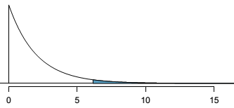- also, it makes sense to have a look at expected $X^2$ for $\alpha = 0.05$, which is $X^2_{\text{exp}} = 5.99$, and $X^2_{\text{exp}} < X^2$ R: ``` obs = matrix(c(3511, 1749, 1818, 1489, 751, 682), nrow=2, ncol=3, byrow=T) dimnames(obs) = list(outcome=c('click', 'new search'), algorithm=c('current', 'test 1', 'test 2')) tot = sum(obs) row.tot = rowSums(obs) col.tot = colSums(obs) exp = row.tot %*% t(col.tot) / tot dimnames(exp) = dimnames(obs) x2 = sum( (obs - exp)^2 / exp ) df = prod(dim(obs) - 1) pchisq(x2, df=df, lower.tail=F) qchisq(p=0.95, df=df) ``` Or we can use chisq.test function ``` test = chisq.test(obs, correct=F) test$expected c('p-value'=test$p.value, test$statistic) ``` ## Links - http://en.wikipedia.org/wiki/Pearson%27s_chi-squared_test#Test_of_independence ## Sources - [OpenIntro Statistics (book)](OpenIntro_Statistics_%28book%29) - [Data Mining (UFRT)](Data_Mining_%28UFRT%29)