Binomial Proportion Confidence Intervals
These are Confidence Intervals for estimating a proportion in the population
- When we sample, we calculate a Point Estimate of the proportion
- We know that due to variance in the Sampling Distribution each time we get different estimates
- How we can expand the point estimate so it’s likely to include the true value?
Normal Approximation
This type of CI makes use of Central Limit Theorem and Normal Approximation of Binomial Distribution
So, for any experiment, let
- $p$ be the true probability
- $n$ be the number of trials
Then
- estimate $p$ as $\hat{p} = \cfrac{\text{success}}{n}$
- and the CI is $\left[\hat{p} - 1.96 \sqrt{p(1-p)/n}; \hat{p} + 1.96 \sqrt{p(1-p)/n}\right]$
Building a Confidence Interval
- We have a sample of $n$ observations: $X_1, …, X_{n}$
- let $\hat{p} = $ fraction of successful $X_i$, i.e. $\hat{p} = \cfrac{\text{# of success}}{n}$
- so we calculate $\hat{p}$ based on the data in the sample
- if all observations are independent and probability of success $p$ is always the same, then Sampling Distribution is Binomial Distribution
- i.e. each $X_i \sim \text{Bernoulli}(p)$, variance $\text{Var}[X_i] = p \cdot (1 - p) = pq$
Parameters of the Sampling Distribution
- $\hat{p}$ is an Unbiased Estimate of $p$: $E[\hat{p}] = p$
- $E[X_i] = p, \hat{p} = \cfrac{1}{n} \sum_{i=1}^n X_i$
- $E[\hat{p}] = E \left[ \cfrac{1}{n} \sum_{i=1}^n X_i \right] = \cfrac{1}{n} \sum_{i=1}^n E [ X_i ] = \cfrac{np}{n} = p$
- $\text{var}[\hat{p}] = \cfrac{p(1-p)}{n}$
- $\text{var}[\hat{p}] = \text{var} \left[ \cfrac{1}{n} \sum_{i=1}^n X_i \right] = \cfrac{1}{n^2} \sum_{i=1}^n \text{var}[X_i] = \cfrac{npq}{n^2} = \cfrac{pq}{n} = \cfrac{p(1-p)}{n}$
- $\text{sd}[ \hat{p} ] = \sqrt{ \cfrac{p \cdot (1 - p)}{n} }$
- Now we use the Normal Approximation (i.e. apply the C.L.T. and calculate that the SD follows Normal Distribution $N \left( \mu=p, \sigma = \sqrt{ \cfrac{p(1-p)}{n} } \right)$)
We want to build CI at level of $\alpha$
- calculate the $z$-score - $1 - 0.5 \cdot \alpha$ percentile of the Standard Normal Distribution
E.g. 95% CI
- $z = 1.96$ and we know that 95% of the values lie in $(-z, +z)$
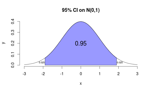
- So only in 5 experiments out of 100 you end up outside of this interval
R code to produce the figure
```carbon x = seq(-3, 3, 0.1) y = dnorm(x) plot(x, y, type='l', bty='n', main='95% CI on N(0,1)') x1 = min(which(x > -1.96)); x2 = max(which(x < 1.96)) polygon(x[c(x1, x1:x2, x2)], c(0, y[x1:x2], 0), col=adjustcolor('blue', 0.4)) text(x=0, y=0.2, labels='0.95', cex=1.5) text(x=c(-2.07, 2.07), y=0.025, labels='0.025', cex=0.6) ```This is called ‘‘95% confidence interval’’ for $p$:
- $\left[\hat{p} - 1.96 \sqrt{p(1-p)/n}; \hat{p} + 1.96 \sqrt{p(1-p)/n}\right]$
- left part - ‘‘lower bound’’
- right part - ‘‘upper bound ‘’
We say that we’re 95% confident that the true value of $p$ is somewhere in this interval.
Margin of Error
Problem: $p$ (to use under the square root) is unknown| | |Solutions:
- use $\hat{p}$ instead of $p$ (we assume it should be close) or
- use $p = q = 0.5$: it maximizes our ‘‘margin of error’’
- <img src=”
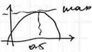 ” />
” /> - margin of error is $\beta = 1.96 \sqrt{p(1-p)/n}$
- <img src=”
Critical Value
Why we chose 95% CI with $\alpha = 0.05$ and not another one?
We can compute any confidence interval using any $\alpha$
- Compute ‘‘critical value’’ $z_{\alpha/2}$ such that “not interesting” areas under the normal curve take $\alpha / 2$
- so the interval will be $\left[-z_{\alpha/2}; z_{\alpha/2}\right]$ and the “interesting” area under the bell curve is $1 - \alpha$
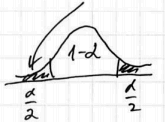
Margin of error is this case is
- $\beta = z_{\alpha/2} \sqrt{p(1-p)/n}$ and, as we know, for $95\%$, $\alpha = 0.025$ and $z_{0.025} = 1.96$
As we see, the CI becomes wider as critical value grows
Assumptions
Note that by using the C.L.T. we assume that:
he central limit theorem applies poorly to this distribution with a sample size less than 30 or where the proportion is close to 0 or 1. The normal approximation fails totally when the sample proportion is exactly zero or exactly one. A frequently cited rule of thumb is that the normal approximation is a reasonable one as long as np > 5 and n(1 − p) > 5;
Examples
Flipping a Beer Cap
Imagine an experiment where we flip a beer cap
- it follows the Binomial Distribution, but we don’t know the true parameter $p$
- say we flipped a beer cap 1000 times and got 576 reds: $\hat{p} = 0.576$
- what is its statistical model? What is $p$ in $\text{Binomial}(1000, p)$?
Let’s build a Confidence Interval for that
- so we estimate $\hat{p} = 0.576$ and $\text{Var}(\hat{p}) = \cfrac{p(1-p)}{n} = \cfrac{p(1-p)}{1000}$
Result:
- 95% CI is $[0.545, 0.607]$
In R:
phat = 0.576
z = qnorm(0.025, mean=0, sd=1, lower.tail=F) // the right tail rather then left
ME = z * sqrt(phat * (1- phat) / 1000) // Margin of error: we replace p by phat
CI = phat + c(-ME, ME) // 0.545, 0.606
Example 2
- Calculate the 90% CI for $p$
- With 60 successes out of 100 trials
```text only phat = 0.6 cl = 0.9 al = (1 - cl) / 2 z = qnorm(al, mean=0, sd=1, lower.tail=F) n = 100
ME = 2 * sqrt(0.5 * 0.5 / n) ci = phat + c(-ME, ME) // [0.52, 0.68] ```
Sample Size
See Also
Sources
- Statistics: Making Sense of Data (coursera)
- OpenIntro Statistics (book)
- https://en.wikipedia.org/wiki/Binomial_proportion_confidence_interval