Binomial Distribution
A binomial distribution is a Discrete Distribution of Random Variables
Intuition
Assume there are $n$ independent experiments
- an event $A$ can either appear with probability $p$ or not appear with probability $q = 1 -p$
- an RV $X$ is the number of experiments in which $A$ appeared
- such experiments are called “Bernoulli Trials”
Using Bernoulli Formula, can calculate that
- the probability of $A$ happening $k$ times out of $n$ trials is
- $P_n(k) = C_n^k \ p^k q^{n-k}$, $0 \leqslant k \leqslant n$
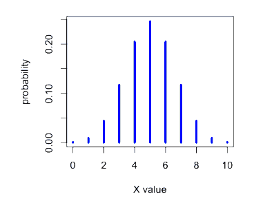
Example
$X \sim \text{Bin}(10, 0.5)$
Main Properties
Expected Value
$E[X] = np$
- let $X$ be the # of independent experiments in which $A$ appeared
- $X = X_1 + X_2 + … + X_n$,
- where $X_i = 1$ if $A$ happened in experiment $i$, and $X_i = 0$ otherwise
- $E[X_i] = 1^2 \cdot p + 0^2 \cdot q = P(A)$
- $E[X] = E \left[ \sum X_i \right] = \sum E[X_i] = np$
Variance
’'’Thm’’’ $\text{Var}[X] = npq$
’'’Proof’’’
- let $X$ be the # of independent experiments in which $A$ appeared,
- $X = X_1 + X_2 + … + X_n$
- $X_i$ are pair-wise independent, i.e. the outcome of one experiment doesn’t depend on the outcome of any other experiment
- thus,
- $\text{Var}[X] = \sum_{i = 1}^n \text{Var}(X_i)$
- $E[X_i] = P(A)$
- $\text{Var}[X_i] = E[X_i^2] - E^2[X_i] = p - p^2 = p(1 - p) = pq$
- since there are $n$ $\text{Var}[X_i]$ then we multiply it by $n$:
- $\text{Var}[X] = npq$
We say that $X$ follows the Binomial Distribution
Examples
Example 1
Произведено 10 независимых испытаний, в каждом из которых вероятность появления события равна 0.6. Найти дисперсию С.В. $X$ - числа появления события в этих испытаниях
- $n = 10, p = 0.6, q = 1 - 0.6 = 0.4 $
- $\text{Var}[X] = npq = 10 \cdot 0.6 \cdot 0.4 = 2.4$
Example 2
Монета брошена два раза. Написать в виде таблицы закон распределения случайной величины $X$ - число выпаданий герба.
$p = 0.5, q = 0.5$
Возможные значения: $x_0 = 0, x_1 = 1, x_2 = 2$
- $P_2(2) = C_2^2 p^2 = 0.25$
- $P_2(1) = C_2^1 pq = 0.5$
- $P_2(0) = C_2^0 q^2 = 0.25$
Normal Approximation
The Bernoulli formula is cumbersome when $n$ is large
- in some cases, the Normal Distribution is a fast way of estimating the binomial probabilities
Binomial Coin Experiment
Link: http://socr.stat.ucla.edu/htmls/SOCR_Experiments.html
- go to the applet page and select “Binomial Coin Experiment”
- set # of trials to 20 and prob of success to 0.13
- we see the theoretical shape
- the applet allows to simulate coin flips and we see that the empirical distribution approaches the theoretical
- what’s the $n$ when we can obtain a unimodal and symmetric distribution?
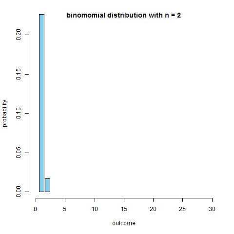
R code to produce the figure
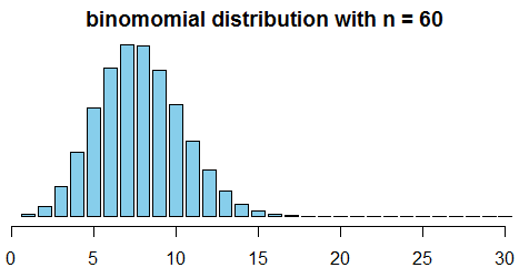
```r require(animation) p = 0.13 max.n = 30 saveGIF({ for (n in 2:130) { x = seq(1, min(n, max.n)) fx = dbinom(x=x, size=n, prob=p) plot(x=NULL, y=NULL, xlim=c(0, max.n), ylim=c(0, 0.2), main=paste("binomomial distribution with n =", n), ylab="probability", xlab="outcome", axes=F) axis(side=1); axis(side=2) bar.width = 0.4 par(xpd=NA) rect(xleft=x-bar.width, xright=x+bar.width, ybottom=0, ytop=fx, col='skyblue') } }, interval=0.1) ```We see that around $n = $ 50-60 it becomes quite symmetric
It’s reasonable to use the Normal Distribution to approximate Binomial
- parameters: $\mu = np, \sigma = \sqrt{npq}$
- note: the sample size should be sufficiently large:
- both $n \cdot p$ and $n \cdot q$ should be at least 10
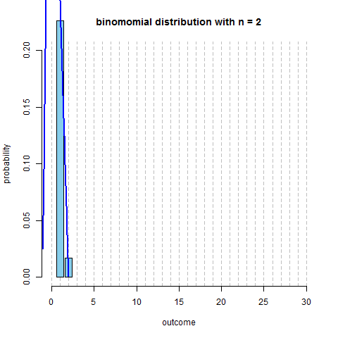
- here’s the same distribution ($p=0.13$, and $n$ increasing) plus $N(np, \sqrt{npq})$
R code to produce the figure
```r saveGIF({ for (n in 2:130) { x = seq(1, min(n, max.n)) fx = dbinom(x=x, size=n, prob=p) plot(x=NULL, y=NULL, xlim=c(0, max.n), ylim=c(0, 0.2), main=paste("binomomial distribution with n =", n), ylab="probability", xlab="outcome", axes=F) par(xpd=FALSE) abline(v=0:30, col='grey', lty=2) axis(side=1); axis(side=2) par(xpd=NA) bar.width = 0.4 rect(xleft=x-bar.width, xright=x+bar.width, ybottom=0, ytop=fx, col='skyblue') fn = dnorm(x=c(-1, 0, 1, x), mean=n*p, sd=sqrt(n*p*(1-p))) xspline(x=c(-1, 0, 1, x), y=fn, lwd=2, shape=1, border="blue") } }, interval=0.1) ```Example
- We want to estimate the prob of observing 59 or fewer smokers in a sample of 400
- the true proportion of smokers is $p=0.20$
- Normal approximation: $\mu = np = 80$, and $\sigma = \sqrt{npq} = 8$
- so use the normal model N(80, 8) to approximate
Compute
- $Z$ score first: $Z = \cfrac{59 - 80}{8} = -2.63$
- The corresponding left tail area is 0.0043.
- the solution with the formula (using the Binomial Distribution) is 0.0041 - approximately equal
Small Intervals
Caution: The normal approximation may fail on small intervals
- Even when the conditions are met, the approximation can still perform poorly
- it’s the case when the range of counts is small
Example:
- want to compute probabilities of observing 69, 70, 71 smokers in 400 people with $p=0.2$
- Binom: 0.0703
- Norm: 0.0476
Reason why:
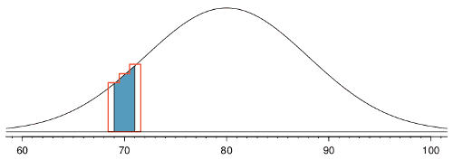
- (source: Figure 3.19 from OpenIntro)
- normal curve + ares between 69 and 71 is shaded
- outlined area - exact binomial probability
- Normal approx is too fine-grained (area for ND is too slim)
- solution in this case is to add extra areas on both sides (-+0.5 and ) - this is called “Continuity Correction” [http://en.wikipedia.org/wiki/Continuity_correction]
Usage
A Sampling Distribution for a population mean follows this distribution
Sources
- Гмурман В.Е., Теория вероятностей и математическая статистика – 9-е издание. М.: Высш. шк., 2003.
- Data Analysis (coursera)
- OpenIntro Statistics (book)
- http://stat.duke.edu/courses/Spring13/sta101.001/slides/unit2lec4H.pdf
- https://en.wikipedia.org/wiki/Binomial_distribution#Normal_approximation