$t$ Distribution
This is a family of Continuous Distributions
- unimodal and bell-shaped, like Normal Distribution
- centered at 0
- has one parameter: degrees of freedom ($\text{df}$)
Origin
Origin (and usage):
- arises when estimating the mean of normally distributed population when
- sample size is small and population standard deviation is unknown
$t$-distribution vs Normal
- for large $\text{df}$ ($\geqslant 100$) $t$-dist closely follows $N(0,1)$
- but even for $\text{df} \geqslant 30$ it’s already almost indistinguishable
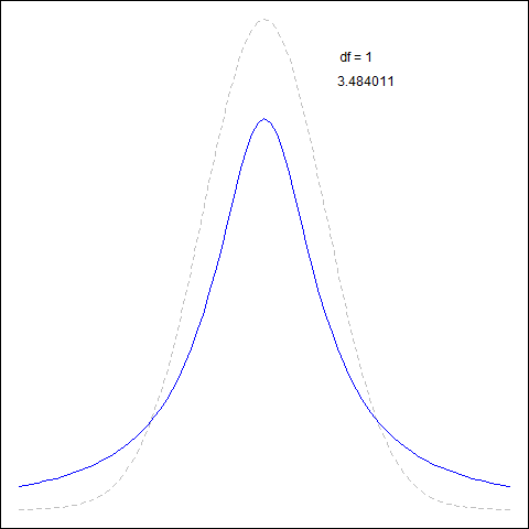
- for $t$ tails are thicker
- so observations are more likely to fall beyond 2$\sigma$ from the mean (than under $N(0,1)$)
- it’s good for t-tests:
- the thick tails are exactly the correction to deal with poorly estimated Standard Error
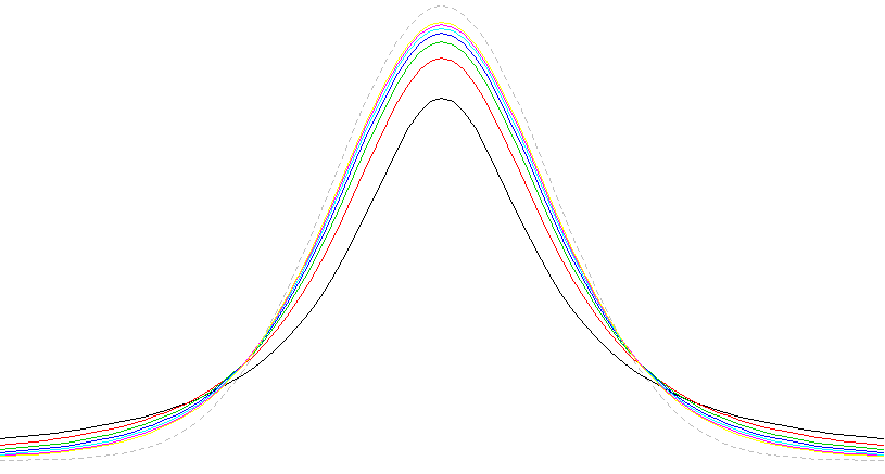
- here, $\text{df}$ is the lowest, and it approaches the normal curse as $\text{df}$ grows
R code to produce the figure
```text only default.par = par() x = seq(-4,4,0.1) n = dnorm(x) library(animation) saveGIF({ par(mar=c(0,0,0,0)) for (i in 1:100) { plot(x, n, type='l', lty=2, col='grey') t = dt(x, df=i) lines(x, t, col='blue') text(1.5, 0.37, paste('df =', i)) text(1.66, 0.35, format(sum(abs(n - t)))) } }, interval=0.1) par(mar=c(0,0,0,0)) plot(x, n, type='l', lty=2, col='grey') for (i in 1:7) { t = dt(x, df=i) lines(x, t, col=i) } par(default.par) ```Sources
- OpenIntro Statistics (book)
- http://projectile.sv.cmu.edu/research/public/talks/t-test.htm