Expected Values for Lotteries
Expected Value is one way to compare lotteries in Decision Trees
Define :
- $EV(l) = \sum_{x \in X} x \cdot p_l(x)$
- $l_1 \ P \ l_2 \iff EV(l_1) > EV(l_2)$ - the preference relation
- $l_1 \ I \ l_2 \iff EV(l_1) = EV(l_2)$ - the indifference relation
So essentially this is the Weighted Sum Model where weights are probabilities
- that helps to establish preferences between lotteries
Advantages
- simple
- good use of information
Disadvantages
- limited to numerical consequences
- no clear rationale
Examples
Example 1
Consider two lotteries
- $l_1$ and $l_2$
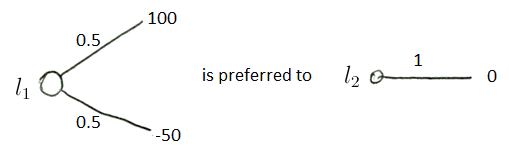
- $l_1$ is a game when you can win 100 euro or lose 50
- $l_2$ is when you don’t play a game
- how to choose whether to play or not (i.e. choose $l_1$ or $l_2$)
- calculate the expected utility: $E(l_1) = 25, E(l_2) = 0$
- so $l_1 \ P \ l_2$
But consider two other lotteries
- $l_3$ and $l_4$
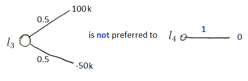
- this time you can win 100k euro or lose 50k
- according to expected value $E(l_3) = 20k > E(l_4) = 0$
- so we should prefer $l_3$ to $l_4$ ($l_3 \ P \ l_4$)
- but the cost of losing is too big - many people cannot afford to play such game
Many people would say
- $l_1 \ P \ l_2$
- but $l_4 \ P \ l_3$
We clearly see that EV is not enough to make a decision
Example 2
The Saint Petersburg Paradox also shows that EV is not a good measure
Expected Value + Variance
When we face such paradoxes we need to add some additional indicators
- such as Variance - to quantify the risk
This is less simple:
- now the problem is bi-objective
- need to use Multi-Objective Optimization techniques
Conclusions
We need to use a different approach