Hypothesis Testing
'’Hypothesis Testing’’ is a framework of testing some assumptions in Inferential Statistics
- a result is ‘‘statistically significant’’ if it’s very unlikely to have happened due to chance alone
Motivation
Suppose we have 2 groups and we observe the difference between them
<img src=”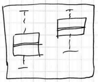 ” />
” />
Question:
- Is this difference significant?
- Could the difference be due to natural variability of the Sampling Distribution?
- Or we have something stronger?
'’Statistical tests’’ (often as well called “Hypothesis tests” or “Tests of Significance”) answer these questions.
Structure of Statistical Test
Summary
- Determine the $H_0$ and $H_A$
- Collect data and calculate a ‘‘test statistic’’
- Calculate the $p$-value
- Make a conclusion based on it and on the context
Step 1: Null and Alternative Hypotheses
- Formulate a hypothesis what you want to test and specify its alternative
Court case analogy: Innocent until proven guilty
- “Innocent” part
- null-Hypothesis $H_0$ (read as “H-naught”)
- it’s a skeptical position or position of no difference
- example: no relationships, no difference, etc
- we assume it’s true
- “Guilty” part:
- alternative hypothesis $H_A$ (or $H_a$ or $H_1$)
- it’s a new perspective
- this is what a researcher wants to establish
- example: relationship, change, difference
And we question we ask is do we have enough evidence to rule out any difference from the $H_0$ that are just due to chance?
Like in a court, we conclude that $H_A$ is true if we have evidence against $H_0$.
Alternatives could be
- one-sided (greater than or less than)
- two-sided (not equal)
So the first step is
- ’'’clearly specify the null and alternative hypotheses’’’
Step 2: Evidence - Test Statistics
- '’The evidence’’ is provided by our data
- We need to summarize the data into a ‘‘test statistics’’: a numerical summary of the data.
A test statistic is made under assumption that $H_0$ is true
So the 2nd step is
- ’'’Collect the data and calculate a test statistic assuming $H_0$ is true’’’
Step 3: $P$-value
- Is the evidence (the test statistics) good enough to reject the $H_0$?
’‘$p$-value’’
- helps us to answer this question: it transforms the test statistic into a probabilistic scale:
- it’s a number between 0 and 1 that quantifiers the strength of evidence against the $H_0$
- formally, $p$-value is a conditional probability of
- observing data favorable to $H_A$ and to the current data set
- given $H_0$ is true
It answers the following question
- Assuming $H_0$ is true, how likely it is to observe a test statistic of this magnitude just by chance?
- And the numerical answer is the $p$-value
The smaller the $p$-value the stronger the evidence against $H_0$
| ’'’Note | ’’’ | - $p$-value cannot be interpreted as how likely it is that the $H_0$ is true. | - $p$-value tells you how unlikely the observed value of the test statistics (and more extreme value) is if the $H_0$ was true. |
So the 3rd step is
- ’'’determine how unlikely the test statistic is if the $H_0$ is true’’’ (or, calculate the $p$-value)
Step 4: Verdict
Based on the $p$-value make a verdict:
- $p$-value is not small
- $\Rightarrow$ conclude that the data is consistent with the $H_0$
- $p$-value is small
- $\Rightarrow$ then we have sufficient evidence against $H_0$ to reject it in favor of $H_A$
- we say “we fail to reject $H_0$”
Strength of the evidence:
- $p < 0.001$ - very strong
- $0.001 \leqslant p < 0.01$ - strong
- $0.01 \leqslant p < 0.05$ - moderate
- $0.05 \leqslant p < 0.1$ - weak
- $p \geqslant 0.1$ - no evidence
The result is statistically significant if the evidence is strong.
The final step:
- ’'’make a conclusion based on the $p$-value’’’ and on the context of the problem (important| ) | |
Common Test Statistics
- $z$-tests - normal, for comparing means
- Binomial Proportion Tests - for comparing proportions, typically approximated by $z$ statistics as well
- $t$-tests - like $z$, but more relaxed (uses $t$-distribution, for comparing means
- $\chi^2$-tests - for normality, variance and goodness of fit
- $F$-tests (ANOVA) - for checking more than 2 samples for equality of means
Terms
- Critical Value
- Power of a test
- Significance level
- $p$-value
- Type I and II Errors (“Decision Errors”)
Decision Errors
| + Summary [http://en.wikipedia.org/wiki/Type_I_and_type_II_errors] || | $H_0$ is true | $H_0$ is false | Reject $H_0$ | align=”center”| Type I error
False positive || align=”center”| Correct outcome
True positive || Fail to reject $H_0$ | align=”center”| Correct outcome
True negative || align=”center”| Type II error
False negative |
Significance Level
- The ‘‘significance level’’ of a test gives a cut-off for how small is small for a $p$-value
- It’s denoted by $\alpha$ and called “desired level of significance”
- $\alpha$ shows how the testing method would perform in repeated sampling
- If $H_0$ is true and you use $\alpha = 0.01$, and you carry out a test repeatedly, with the same size of a sample each time, you will reject $H_0$ 1% of the time, and not reject 99% of the time
- If $\alpha$ is too small, you may never reject $H_0$, even if the true value is very different from the $H_0$
Choosing $\alpha$
- traditionally, $\alpha=0.05$
- if making Type I Errors is dangerous, or especially costly, choose small $\alpha$
- in this case we want very strong evidence to support $H_A$ before rejecting $H_0$
- if Type II Errors are more costly, then take higher $\alpha$, e.g. $\alpha=0.1$
- here we’re careful about failing to reject $H_0$ when it’s false
Robustness
A statistical test is ‘‘robust’’ if the p-value is approximately correct even if some conditions aren’t fully satisfied
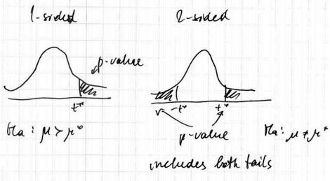
One-Sided vs Two-Sided
Alternative hypotheses $H_A$ could be one-sided or two-sided
- if it’s one-sided we look only at the corresponding tail of our Sampling Distribution
- otherwise we look at both tails
Consider the following one-sample $z$-test for means:
One-Sided
- $H_0: \mu = \mu_0, H_A: \mu > \mu_0$
- $\mu_0$ is called the “null value” because we assume it under $H_0$
- i.e. we want to check if population mean is larger than some value
- under the Normal Model we calculate the $z$-score and corresponding $p$ value of the right tail

- (source: OpenIntro, figure 4.16)
Analogously, for
- $H_0: \mu = \mu_0, H_A: \mu < \mu_0$
- we calculate the $p$-value based on the left tail

- (source: OpenIntro, figure 4.16. modified)
Two-Sided
Two-Sided alternative hypotheses looks at both left and right tails. E.g.
- $H_0: \mu = \mu_0, H_A: \mu \ne \mu_0$

- (source: OpenIntro, figure 4.19, modified)
- if this case, we reject $H_0$ if the test statistics gets under any of the shaded tails
- i.e. the $p$-value is (typically) twice bigger than for one-sided tests
Advice for Hypothesis Testing
$p$-values
- Don’t misinterpret $p$-values (see what p-values say and what don’t)
- A $p$-value is a measure of the strength of the evidence - so don’t forget to report it
Data Collection
Data Collection matters
- Sample wisely:
- use randomization to avoid flaws and biases
Two-Sided Tests
Always try to use 2-sided tests
- Unless you’re really sure you need one direction
- $p$-value for one-sided test is 0.5 of p-value of 2-sided
One-sided hypotheses are allowed only before seeing the data
- it’s never good to change 2-sided to 1-sided after observing the data
- it can cause twice more Type I errors (False positives - i.e. rejecting $H_0$ when it’s true)
Practical Significance
Statistical significance $\neq$ practical significance
- the larger the $n$, the smaller $p$-value
- A large $p$-value doesn’t necessarily mean that the $H_0$ is true, there might be not enough power to reject it.
Small $p$-values can occur (in order of significance:)
- '’by chance’’
- data collection is biased
- violations of the conditions
- $H_0$ is false (the last one| - so be more careful about those above!) | | So
- If multiple tests are carried out, some are likely to be significant by ‘'’chance alone’’’
- If $\alpha = 0.05$ we expect significant results 5% of the time, even when the $H_0$ is ‘'’true’’’
- $\Rightarrow$ be suspicious if you see only a few significant results when many tests have been carried out
Data Snooping
- The test results are not reliable if the statements of the hypotheses are suggested by data.
- This is called ‘‘data snooping’’ - So hypotheses should be specified before any data is collected
General Advice
- Start with Explanatory Data Analysis e.g. using Plots and Summary Statistics
- watch for skewed distributions, Outliers, etc
- before using some test statistics, make sure the corresponding assumptions about the data hold
Relationship with Confidence Intervals
Some hypothesis can be checked with Confidence Intervals
- e.g. if the null value (the value under $H_0$) is included in the CI, then $p$-value is greater than $\alpha$ and we fail to reject $H_0$
See Also
Sources
- Statistics: Making Sense of Data (coursera)
- OpenIntro Statistics (book)
- http://en.wikipedia.org/wiki/Statistical_hypothesis_testing