Join Ordering
This is a part of Physical Query Plan Optimization procedure
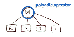
In a Logical Query Plan the order of joins is not fixed
- there we assumed that this is a polyadic operation
Example
- $R(A, B), S(B, C), T(C, D), U(D, A)$
- want $R \Join S \Join T \Join U$
Importance of Orderings
But physical join operators#Join) are binary
- Order becomes important how can we order these joins?
- $R \Join S \Join T \Join U \equiv$
- $((R \Join S) \Join T) \Join U \equiv$
- $(R \Join S) \Join (T \Join U) \equiv$
- $((R \Join T) \Join U) \Join S \equiv$
- $…$
- A lot| (note that natural join is possible even if there are no matching tuples) Recall that Join is the most expensive operation
- need to carefully choose the order
Example
- given: $R(A, B), S(B, C), T(A, E)$
- statistics:
- $B(R) = 50, B(S) = 50, B(T) = 50$
- $B(R \Join S) = 150$
- $B(S \Join T) = 2500$ ($S$ and $T$ don’t have anything in common - so it’s a cartesian product)
- $B(R \Join T) = 200$
- assume ideal case: everything can be done with one-pass join#One-Pass_Join) algorithm
- i.e. we have # of free buffers $M = 51$
- what’s the best ordering for $R \Join S \Join T$?
$R \Join (S \Join T)$
- $S \Join T$ - the largest
- cost:
- $B(R) +$ (read $B$ once)
- $B(S \Join T) +$ (too big intermediate result - need to flush to disk)
- $B(S) + B(T)$
- = 2650
$S \Join (R \Join T)$
- cost: $B(S) + B(R \Join T) + B(R) + B(T) = 350$
$(R \Join S) \Join T$
- cost: $B(T) + B(R \Join S) + B(R) + B(S) = 300$
So we see that the order is indeed important
- we want to avoid computing big subresults that we don’t need afterwards
Optimization Problem
Possibly Orderings
We see that we need to enumerate all possible join orderings
- in how many ways we can put ()s?
- how many permutations are there?
$\Rightarrow$ the number of possible orderings is $n| \times T(n)$
- $n!$ - number of ways to permute $n$ relations
- $T(n)$ ways to create a binary tree over $n$ leaf nodes
- $T(1) = 1, T(n) = \sum_{i = 1}^{n - 1} T(i) \times T(n - 1)$
The resulting space is super-exponential:
| $n$ | 2 | 3 | 4 | 5 | 6 | 7 | 8 || $n! \times T(n)$ | 2 | 12 | 120 | 1680 | 30 240 | 665 580 | 17 297 280 | The query optimization must not take longer than the most stupid and naive way of executing it
- so we disregard the option of trying all possible orderings and infeasible
Types of Ordering
Instead of listing all possible orderings we will consider only one of the following types
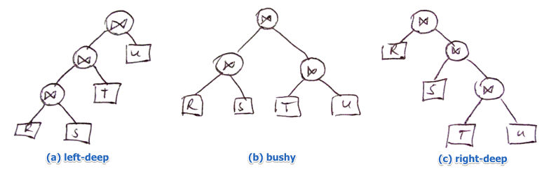
- (a): $((R \Join S) \Join T) \Join U$
- (b): $(R \Join S) \Join (T \Join U)$
- (c): $R \Join (S \Join (T \Join U))$
a typical query optimizer usually looks only at left-deep join orderings
- (a) $\approx$ (c), but there are subtle implementation-wise differences
- (like being able to pipeline some results, etc)
- still, there are $n!$ possible orderings (and it’s still exponential)
This is an Optimization Problem. Solutions:
- some heuristics
- Branch and Bound
- Dynamic Programming
- Greedy Algorithms
Greedy Algorithm
Always make locally optimal choices
Algorithm
- start with two relations that give the best cost
- for remaining relations choose the cheapest relation to join with the result-so-far
- repeat until there are no relations left
That generates a left-deep join ordering
Not Always Optimal
Of course since it uses some kind of Local Search, it may stuck in local optima
Suppose:
- join on $R(A, B), S(B, C), T(C, D), U(A, D)$
- costs:
- $\underbrace{B(R \Join S) = 100}{(1)}, \underbrace{B((R \Join S) \Join T)) = 2000}{(2)}$
- $\underbrace{B(R \Join U) = 200}{(3)}, \underbrace{B((R \Join U) \Join T)) = 1000}{(4)}$
- Greedy algorithm will select
- $((R \Join S) \Join T) \Join U$
- $(1)$ gives us better cost than $(3)$
- alternative ordering:
- $((R \Join U) \Join T) \Join S$
- $(3)$ is not better than $(1)$, but $(4)$ (given $(3)$) is better than $(2)$ (given $(1)$)
- 900 I/Os saved
|
Exercises