PROMETHEE

PROMETHEE

This is a method from the family of outranking (i.e. based on pair-wise comparison) MCDA methods.

PROMETHEE stands for Preference Ranking Organization METHod for Enrichment Evaluation

Notation:

• $A = {a_1, …, a_n}$ - set of alternatives
• $F = {f_1, …, f_q}$ - set of criteria (assume we maximize everything)

Note that since we perform pair-wise comparisons, it may become computationally very expensive

There are four steps:

1. Compute Uni-Criterion Preferences
2. Compute Preference Matrix
3. Compute Net-Flow Scores
4. Rankings
   • Complete: PROMETHEE II
   • Partial: PROMETHEE I

Parameters for a problem (a decision maker needs to specify them)

• the type of preference function $P_k$ used for each criterion $f_k$
• weight $w_k$ for each criterion $f_k$

Uni-Criterion Preferences

we calculate the differences in all criteria for all pairs of alternatives:

• $\forall a_i, a_j \in A: d_k(a_i, a_j) = f_k(a_i) - f_k(a_j)$
• since we assume that we maximize everything, the bigger the difference, the better the first alternative is

The resulting value should be normalized:

• we apply a (pre-defined for each criteria $f_k$) preference function $P_k$ to each difference
• $\pi_k = P_k \big[ d_k(a_i, a_j) \big]$
• this transforms the difference into the preference degree

Preference Functions

There are 6 preference functions:

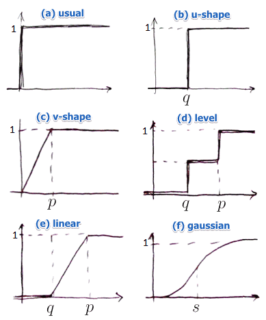
Basic Shapes

• (a) usual preference function
  • as soon as see any difference, the preference is 1
  • no need to specify any parameters
  • this function is very sensitive
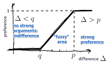
• (b) $u$-shape function
  • difference needs to exceed a certain threshold $q$
  • (a) and (b) are typically used for qualitative scales
• (c) $v$-shape
  • with strong preference threshold $p$
• (d) level
• (e) linear
  • same as (c) but with sensitivity threshold $q$
  • 
• (f) $v$-shape

Choosing a shape is already a decision

Preference Matrix

At this step we compute global preference degrees

• that is, for each pair $a_i, a_j$ compute:
• $\pi(a_i, a_j) = \sum_{k=1}^q w_k \cdot \pi_k (a_i, a_j)$
• global preference degree is a weighted sum of uni-criteria preferences

Consequences:

• $\pi(a_i, a_i) = 0$
  • the preference of element $a$ with itself is always 0
  • $\pi(a_i, a_i) = \sum_{k=1}^q w_k \cdot \pi_k (a_i, a_i) = \sum_{k=1}^q w_k \cdot P_k \big[ \underbrace{d_k(a_i, a_i)}_{= \ 0} \big] = 0$
• $\pi(a_i, a_j) \geqslant 0$
  • the preference degree is always positive
  • $\pi(a_i, a_j)$ is a weighed sum of $\pi_k$ which are always positive
  • this is because the preference functions always return positive values
• $\pi(a_i, a_j) + \pi(a_j, a_i) \leqslant 1$
  • ’'’todo’’’

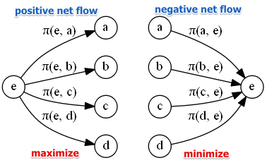
Net Flow Scores

For each $a_i, a_j \in A$ we compute net flow scores

• $\Phi^+(a_i) = \cfrac{1}{n-1} \sum_{a_j \in A} \pi(a_i, a_j)$
  • '’positive outranking net flow’’
  • “strengths” of an alternative, how an alternative outranks others
  • want to maximize it
• $\Phi^-(a_i) = \cfrac{1}{n-1} \sum_{a_j \in A} \pi(a_j, a_a)$
  • '’negatives outranking net flow’’
  • “weaknesses” of an alternative, how an alternative is outranked by others
  • want to minimize it

The values are normalized:

• $\Phi^+(a_i) \in [0, 1]$ and
• $\Phi^-(a_i) \in [0, 1]$

The flow score is computed as difference between the positive flow and negative flow

• $\Phi(a_i) = \Phi^+(a_i) - \Phi^-(a_i) \in [-1, 1]$ and

'’Uni-criteria flow’’

• flow computed with respect to only one criteria $f_k$
• $\Phi_k(a) = \cfrac{1}{n-1} \sum_{b \in A} [ P_k(a, b) - P_k(b, a) ]$

Ranking

PROMETHEE I

Partial Order Ranking:

• ranking based only on $\Phi^+(a_i)$ and $\Phi^-(a_i)$ (not on the aggregated flow score)
• let $P^+$ denote the preference of $\Phi^+$
  • $a_i \ P^+ \ a_j \iff \Phi^+(a_i) > \Phi^+(a_j)$ (want to maximize $\Phi^+$)
• let $P^-$ denote the preference of $\Phi^-(a_i)$
  • $a_i \ P^- \ a_j \iff \Phi^+(a_i) < \Phi^+(a_j)$ (want to maximize $\Phi^-$)
• $a_i \ P \ a_j \iff a_i \ P^+ \ a_j \land a_i \ P^- \ a_j$
  • i.e. $a_i$ is preferred to $a_j$ only in case of Unanimity between $\Phi^+$ and $\Phi^-$
• if there is no unanimity, $a \ J \ b$
  • $a$ is not comparable to $b$
  • in this case it’s up to the decision maker to decide what to do with these alternatives

PROMETHEE II

This gives a completely ordered preference structure

• i.e. there’s no $J$ relation

Define:

• preference as $a_i \ P \ a_j \iff \Phi(a_i) > \Phi(a_j)$
• indifference as $a_i \ I \ a_j \iff \Phi(a_i) = \Phi(a_j)$

These relations are transitive and complete

Properties

Justification

; The PROMETHEE property:

• the netflow score $\Phi(a_i)$ is a centered score $s_i$ ($\forall i$) that minimizes the following $Q$:
• $Q = \sum_{i=1}^n \sum_{j=1}^n \big[ (s_i - s_j) - (\pi_{ij} - \pi_{ji}) \big]^2 $
• i.e. $Q$ is the sum of squared deviation and we want to minimize it
• proof: PROMETHEE/Properties#The PROMETHEE Property

Property 1

; $\Phi(a_i) \in [-1, 1]$ Easy to see that by the way we construct $\Phi(a_i)$

Property 2

Want to show that $\sum_{i = 1}^N \Phi(a_i) = 0$

• $N$ - the number of alternatives
• that can be shown by induction
• proof: PROMETHEE/Properties#Property 2

Preferential Independence

PROMETHEE respects the Preferential Independence hypothesis

• PROMETHEE/Properties#Preferential Independence

Arrow’s Impossibility Theorem

Recall that according to the theorem all 5 conditions cannot be satisfied at the same time.

• Independence to Third Alternatives, due to pair-wise comparisons is not respected (shown below in PROMETHEE/Rank Reversal)
• but it satisfies all the rest
• The Monotonicity property is satisfied PROMETHEE/Properties#Monotonicity

Rank Reversal

A rank reversal happens if:

• $\pi_{ij} \geqslant \pi_{ji}$ but in spite of that $\Phi(a_i) \leqslant \Phi(a_j)$
• the main article: PROMETHEE/Rank Reversal

GAIA

PROMETHEE gives you scores and you can compute complete and partial rankings

• GAIA is a tool for visualizing, complimentary to PROMETHEE
• GAIA = Geometrical Analysis for Interactive Assistance

We can represent each alternative as a vector:

• we can represent an alternative as a vector of $q$ components:
  • $[f_1(a_i), …, f_q(a_i)]$
  • but in this space we have different scales - and things are not easy to compare
• we can use the netflow score, which is a value in $[-1, 1]$
  • $\Phi(a_i) = \sum_{k=1}^{q} w_k \cdot \phi_k(a_i)$
  • where $\Phi_k(a_i) = \cfrac{1}{n-1} \sum_{a_j \ne a_i} \big[ \pi_k(a_i, a_j) - \pi_k(a_j, a_i) \big] $
• so we can represent every alternative $a_i$ as a vector $[\Phi_1(a_i), …, \Phi_k(a_i)]$ in $q$ dimensional space.

But $q$ dimensional space is really hard to visualize

• GAIA does that
• it applies Principal Component Analysis for projecting $q$-dim space to 2-dim space

$\delta$

• some information is lost during the projection, and the $\delta$ coefficient shows how much information is retained on the plane
• $\delta$ is the ratio between the projected variance and the initial variance
• $\delta \geqslant 70\%$ is good

Example

Consider a “Buying a new car” example (from D-Sight [http://www.d-sight.com/learning-center/articles/buying-new-car])

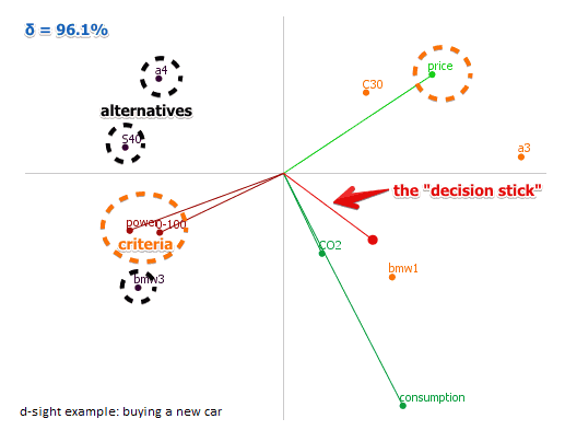
• points are alternatives
• lines with points at the end are criteria
• the red stick is a ‘‘decision stick’’ - the projection of weights to the plain

Based on a GAIA plane can make some observations:

• there are conflicting criteria: ones that point in the opposite directions
• there are also criteria that are in synergy: they point in the same direction
• 
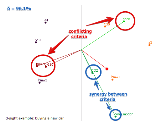
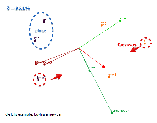
• some criteria are close to each other in 2-dim space - they also must be close in the $q$-dim space, so they should have similar profiles
• 
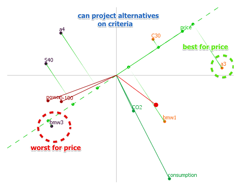
• it is also interesting to see the position of alternatives with respect to criteria: to project each as see which one is the best, worst, etc
• 
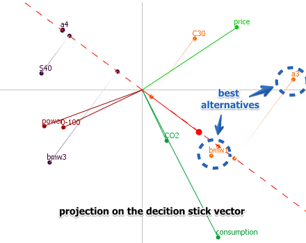
• and finally, the projection on the decision stick vector shows what are the best alternatives
• 

Example: Plant Location Problem

Evaluation Table

First we establish the following evaluation table:

| | # engineers | power | cost | maintenance | village | security | Italy | 75 | 90 | 600 | 5.4 | 8 | 5 || Belgium | 65 | 58 | 200 | 9.7 | 1 | 1 || Germany | 83 | 60 | 400 | 7.2 | 4 | 7 || Sweden | 40 | 80 | 1000 | 7.5 | 7 | 10 || Austria | 52 | 72 | 600 | 2 | 3 | 8 || France | 94 | 96 | 700 | 3.6 | 5 | 6 || | min | max | min | min | max | max |

• red

  color - worst value in column

• blue

  color - best value in column

Pair-wise Comparison

• start with 2 alternatives and consider only 1 criteria at a time
• for example, $G$ermany and $A$ustria:
• cost is better in $G$: 400 vs 600
  • what does it mean?
  • need to normalize this difference to [0, 1] scale - to be able to qualify the difference

Unic. pref

0.25

-200

Germany

83

60

400

7.2

4

7

Engineers

Power

Cost

Maint.

Village

Security

Austria

52

72

600

2

3

8

-31

12

-5.2

-1

1

Unic. pref

1

0.75

1

0.3

0.63

Global Preference Degree

Next step: compute global preference degree for all pairs of alternatives

• assuming a decision maker provides the weights
• eng: 0.1, pow: 0.2, cost: 0.2, maint: 0.1, village: 0.15, security: 0.15 (sum = 1)
• $\pi(A, G) = 1 \cdot 0.1 + 0.75 \cdot 02 + 1 \cdot 0.1 + 0.3 \cdot 0.15 + 0.63 \cdot 0.15 = 0.498$
• $\pi(G, A) = 0.25 \cdot 0.4 = 0.05$
• the closest the $\Pi$ value to 1, the move preferred one alternative to another is

We do this for all pairs and build a preference matrix

Italy

Belgium

Germany

Sweden

Austria

France

Italy

0

0.28

0.23

0.24

0.09

0.22

Belgium

0.27

0

0.4

0.3

0.27

0.5

Germany

0.22

0.19

0

0.3

0.05

0.43

Sweden

0.43

0.55

0.33

0

0.25

0.25

Austria

0.46

0.55

0.49

0.34

0

0.46

France

0.23

0.4

0.26

0.39

0.12

0

Net Flow Scores

Next we compute the positive and negative net flow scores:

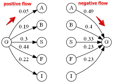
• positive flow: strengths, has to be maximized
• negative flow: weaknesses, has to be minimized

Then we calculate if on average $G$ is better than the rest:

• $\Phi^+(G) = 0.238$ (avg of all $\Pi(G, X)$)
• $\Phi^-(G) = 0.334$ (avg of all $\Pi(X, G)$)
• the total score: $\Phi(G) = \Phi^+(G) - \Phi^-(G) = -0.1 \in [-1, 1]$

PROMETHEE II ranking

: ranking the alternatives based on their netflow scores

rank

alternative

$\Phi(G)$

$\Phi^+(G)$

$\Phi^-(G)$

1

Austria

0.302

0.458

0.156

2

Sweden

0.049

0.363

0.314

3

Belgium

-0.041

0.347

0.397

4

Germany

-0.096

0.238

0.334

5

France

-0.099

0.274

0.373

6

Italy

-0.115

2.11

0.326

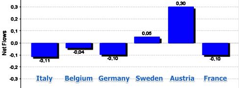
Note that this is a complete ranking:

• you can always say which alternative is better

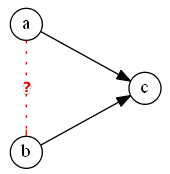
PROMETHEE I ranking

| | $\Phi^+$ | $\Phi^-$ | $a$ | 0.8 | 0.1 || $b$ | 0.5 | 0.05 || $c$ | 0.1 | 0.8 | for both $\Phi^+$ and $\Phi^-$ (applying the Unanimity principle)

• $a \ P \ c$
• $b \ P \ c$

Cannot say anything about $a$ and $c$

• for $\Phi^+$: $a \ P \ b$
• for $\Phi^-$: $b \ P \ a$

Sources

• Decision Engineering (ULB)
• An Introduction to Multicriteria Decision Aid: The PROMETHEE and GAIA Methods, Yves De Smet, Karim Lidouh, 2013