System of Linear Equations
The fundamental problem of Linear Algebra is solving a system of Linear Equations.
- A system of linear equations is a system of first order equations with multiple unknowns.
$A \mathbf x = \mathbf b$
Matrix View
Suppose we have a system with $m$ equations and $n$ unknowns:
$\left{\begin{matrix}
a_{11} x_1 + a_{12} x_2 + \ … \ + a_{1n} x_n = b_1\
a_{21} x_1 + a_{22} x_2 + \ … \ + a_{2n} x_n = b_2\
\vdots
a_{m1} x_1 + a_{22} x_2 + \ … \ + a_{mn} x_n = b_m\
\end{matrix}\right.$
The coefficients of the unknowns form a Matrix - a rectangular array of numbers:
- $A = \begin{bmatrix} a_{11} & a_{12} & … & a_{1n}\ a_{21} & a_{22} & … & a_{2n}\ \vdots & \vdots & \vdots & \vdots \ a_{m1} & a_{m2} & … & a_{mn} \end{bmatrix}$
- We call this matrix $A$, it’s $m \times n$ matrix: with $m$ rows and $n$ columns
The unknowns themselves form a column vector $\mathbf{x}$, and the … form a column vector $b$
- $\mathbf{x} = \begin{bmatrix}
x_1
x_2
\vdots
x_n
\end{bmatrix}$, $\mathbf{b} = \begin{bmatrix} b_1
b_2
\vdots
b_m
\end{bmatrix}$, - they’re both column vectors, $\mathbf{x}$ has size $n$, and $\mathbf{b}$ has size $m$
- can write them as rows using the transposition notation: $\mathbf{x} = [x_1, x_2, …, x_n]^T$ (but they still remain column vectors)
So the system of linear equations can be expressed in a matrix form as $A\mathbf{x} = \mathbf{b}$
Geometry of Linear Equations
Suppose we have the following system of linear equations:
$\left{\begin{matrix} 2x - y = 0\ -x + 2y = 3 \end{matrix}\right.$
Matrix form:
- $\begin{bmatrix}
2 & -1 \
-1 & 2
\end{bmatrix} \begin{bmatrix}
x \ y
\end{bmatrix} = \begin{bmatrix} 0 \ 3
\end{bmatrix}$
We can see this in two possible ways:
- as a crossing of lines (hyperplanes) - the row picture
- as vectors - the column picture
Row Picture
We have two lines:
- $2x - y = 0$, $-x + 2y = 3$
- plot them, and the point where they cross is the solution $\mathbf{x}$
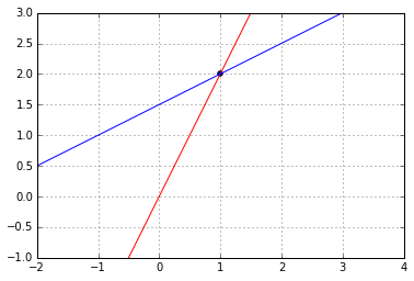
The solution is $[x, y]^T = [1, 2]^T$
For 3 and more dimensions, we have (hyper)planes instead of lines.
- But it’s the same: we want to find a point where they cross
- File:Secretsharing_3-point.svg
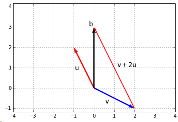
Column Picture
We have two vectors:
- $x \begin{bmatrix}
2 \
-1
\end{bmatrix} + y \begin{bmatrix} -1 \ 2 \end{bmatrix} = \begin{bmatrix} 0 \ 3 \end{bmatrix}$
We need to combine first two vectors $v = \begin{bmatrix} 2 \ -1 \end{bmatrix}$ and $u = \begin{bmatrix} -1 \ 2 \end{bmatrix}$ so they form $\begin{bmatrix} 0 \ 3 \end{bmatrix}$
I.e. we want to find a Linear Combination of these columns.
- From the vector picture we know that the solution is $[1, 2]^T$, so let’s take
-
so we take 1 of vector $\mathbf u$ and 2 of vector $\mathbf v$ and end up at exactly $\mathbf b$
Python Code
Python code to reproduce the figures
```python import matplotlib.pylab as plt import numpy as np class Line: def __init__(self, slope, intercept): self.slope = slope self.intercept = intercept def calculate(self, x1): x2 = x1 * self.slope + self.intercept return x2 line1 = Line(2, 0) line2 = Line(0.5, 1.5) a = np.array([-6, 6]) plt.plot(a, line1.calculate(a), color='red', marker='') plt.plot(a, line2.calculate(a), color='blue', marker='') plt.scatter([1], [2]) plt.grid() plt.axis('equal') plt.ylim([-1, 3]) plt.xlim([-1, 3]) ``` ```python import matplotlib.pylab as plt plt.axis('equal') plt.quiver([0, 0, 0], [0, 0, 0], [-1, 2, 0], [2, -1, 3], color=['red', 'blue', 'black'], angles='xy', scale_units='xy', scale=1) plt.quiver([2], [-1], [-2], [4], color='red', width=0.005, scale=1, angles='xy', scale_units='xy') plt.grid() plt.ylim([-2, 5]) plt.xlim([-4, 4]) plt.show() ```Solving the System
How we can solve the system $A \mathbf x = \mathbf b$?
- The easiest way: Gaussian Elimination - elimination of variables
- this is the row picture
Vector Solution: the solution found with the column picture
Matrix Solution
- if $A$ is non-singular and invertible, then to find $\mathbf x$ multiply $\mathbf b$ by the inverse of $A$: $\mathbf x = A^{-1} \mathbf b$
- if $\mathbf b \in C(A)$ - Column Space of $A$
- this is especially important when the number of columns $n$ is less than the number of rows $m$
Solving $A \mathbf x = \mathbf 0$
Such systems are called ‘‘homogeneous’’ - see Homogeneous Systems of Linear Equations
Complete Solution to $A \mathbf x = \mathbf b$
Let $A$ be $n \times m$ matrix of rank $r$
- we know that the system has a solution if $\mathbf b \in C(A)$
Steps:
- reduce $A$ to Row Reduced Echelon Form
- set all free variables to 0 and solve - get $\textbf x_p = \textbf x_\text{particular}$
- then solve $A \mathbf x_n = \mathbf 0$ - get all $\mathbf x_n$ - all $\mathbf x$ that solve the homogeneous system
- Then find all other solutions: they are $\mathbf x = \textbf x_p + \mathbf x_n$
- this solution is called ‘‘the complete solution’’
- why? $A \mathbf x_p = \mathbf b$ and $A \mathbf x_n = \mathbf 0$. Add them and get $A \cdot (\mathbf x_p + \mathbf x_n) = \mathbf b + \mathbf 0 = \mathbf b$
- so we can the solution as the Nullspace $C(A)$ but shifted away from the origin by $x_p$
- note that this solution doesn’t form a subspace
General Case, $A \mathbf x = \mathbf b$
Let $A$ be $m \times n$ matrix of rank $r$
- $m$ - rows, $n$ - cols
- $r \leqslant m$, $r \leqslant n$
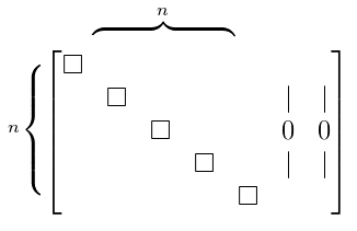
Full Column Rank
Full rank = $r$ is as big as it can be
- suppose that $n \leqslant m$, i.e. the number of columns is smaller than the number of rows
- so full column rank matrix = $r = n$
- there’s a pivot in every column, $n$ pivots $\Rightarrow$ no free variables
Nullspace $N(A)$?
- there are no free variables to consider
- so $N(A) = { \ \mathbf 0 \ }$
Solution to $A \mathbf x = \mathbf b$:
- if the solution exists (i.e. $\mathbf b \in C(A)$) then this solution is unique
- so we have either 0 solutions or 1
- No solution? Can approximate it with Normal Equation (That would be the Least Squares solution)
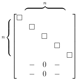
Full Row Rank
- Now suppose that $m \leqslant n$ and $r = m$
- so every row has a pivot, but only $r$ columns have pivots, the remaining $n - r$ don’t
- so there are $r$ pivot columns, and $n - r$ free columns
for which $\mathbf b$ we can solve $A \mathbf x = \mathbf b$?
- there are no zero rows, so can solve the system for any $\mathbf b$
Full Rank
- If our $A$ is square, $m = n = r$
- then there’s always a solution, and $A$ is called ‘‘invertible’’
- $N(A) = { \ \mathbf 0 \ }$ - there’s only one unique solution
=== $r < m$ and $r < n$ ===
- $A \mathbf x = \mathbf 0$ always have a solution - there’s always something in the Nullspace $N(A)$ of $A$ apart from the zero-vector
- reason: there are always free variables and we can assign any non-zero values to them and solve the homogeneous system
Zero or $\infty$ solutions
Sources
- Linear Algebra MIT 18.06 (OCW)
- Курош А.Г. Курс Высшей Алгебры
- http://en.wikipedia.org/wiki/System_of_linear_equations