$\require{cancel}$
Normal Equation
- This is a technique for computing coefficients for Multivariate Linear Regression.
- the problem is also called OLS Regression, and Normal Equation is an approach of solving it
- It finds the regression coefficients analytically
- It’s an one-step learning algorithm (as opposed to Gradient Descent)
Multivariate Linear Regression Problem
Suppose we have
- $m$ training examples $(\mathbf x_i, y_i)$
- $n$ features, $\mathbf x_i = \big[x_{i1}, \ … \ , x_{in} \big]^T \in \mathbb{R}^n$
- We can put all such $\mathbf x_i$ as rows of a matrix $X$ (sometimes called a design matrix)
- $X = \begin{bmatrix}
- \ \mathbf x_1^T - \ \vdots \
- \ \mathbf x_m^T - \ \end{bmatrix} = \begin{bmatrix} x_{11} & \cdots & x_{1n} \ & \ddots & \ x_{m1} & \cdots & x_{mn} \ \end{bmatrix}$
- the observed values: $\mathbf y = \begin{bmatrix} y_1 \ \vdots \ y_m \end{bmatrix} \in \mathbb{R}^{m}$
- Thus, we expressed our problem in the matrix form: $X \mathbf w = \mathbf y$
- Note that there’s usually additional feature $x_{i0} = 1$ - the slope,
- so $\mathbf x_i \in \mathbb{R}^{n+1}$ and $X = \begin{bmatrix}
- \ \mathbf x_1^T - \
- \ \mathbf x_2^T - \ \vdots \
- \ \mathbf x_m^T - \ \end{bmatrix} = \begin{bmatrix} x_{10} & x_{11} & \cdots & x_{1n} \ x_{20} & x_{21} & \cdots & x_{2n} \ & & \ddots & \ x_{m0} & x_{m1} & \cdots & x_{mn} \ \end{bmatrix} \in \mathbb R^{m \times n + 1}$
Thus we have a system
- $X \mathbf w = \mathbf y$
- how do we solve it, and if there’s no solution, how do we find the best possible $\mathbf w$?
Least Squares
There’s no solution to the system, so we try to fit the data as good as possible
- Let $\mathbf w$ be the best fit solution to $X \mathbf w \approx \mathbf y$
- we’ll try to minimize the error $\mathbf e = \mathbf y - X \mathbf w$ (also called residuals)
- we take the square of this error, so the objective is
- $J(\mathbf w) = | \mathbf e |^2 = | \mathbf y - X \mathbf w |^2$
Minimization
So our problem is
- $\hat{\mathbf w} = \operatorname{arg \, max}\limits_{\mathbf w} J(\mathbf w) = \operatorname{arg \, max}\limits_{\mathbf w} | \mathbf y - X \mathbf w |^2$
- let’s expand $J(\mathbf w)$:
- $J(\mathbf w) = | \mathbf y - X \mathbf w |^2 = ( \mathbf y - X \mathbf w )^T ( \mathbf y - X \mathbf w ) = \mathbf y^T \mathbf y - (X \mathbf w)^T \mathbf y - \mathbf y^T (X \mathbf w) + (X \mathbf w)^T (X \mathbf w) = \ …$
- $… \ = \mathbf y^T \mathbf y - 2 \mathbf w^T X^T \mathbf y + \mathbf w^T X^T X \mathbf w$
- now minimize $J(\mathbf w)$ w.r.t. $\mathbf w$:
-
$\frac{\partial J(\mathbf w)}{\partial \mathbf w} = - 2 X^T \mathbf y + 2 X^T X \mathbf w \mathop{=}\limits^ \mathbf 0$
-
- $X^T X \mathbf w = X^T \mathbf y$ or
- the solution:
- $\mathbf w = (X^T X)^{-1} X^T \mathbf y = X^+ \mathbf y$
- where $X^+ = (X^T X)^{-1} X^T$ is the Pseudoinverse of $X$
Linear Algebra Point of View
In Linear algebra we typically use different notation
- Instead of $X$ we use $A$ - it’s a System of Linear Equations that is very tall and thin
- so we have an $m \times n$ matrix $A$ s.t. $m > n$ -
- we need to solve the system $A \mathbf x = \mathbf b$
- if $\mathbf b \not \in C(A)$ (Column Space) then there’s no solution
- how to find an approximate solution? Project onto $C(A)$
- it also gives the Normal Equation
Projection onto $C(A)$
Suppose we have a matrix $A$ with out observations
- the system $A \mathbf x = \mathbf b$ has no solution
- We project $\mathbf b$ on the Column Space $C(A)$
- how do we do it? $C(A)$ is all the combinations of columns in $A$, so they form a hyperplane in $\mathbb R^m$
- $\mathbf b$ is not on this hyperplane - otherwise we would not need to project on it
Normal Equation:
- so we have $A \mathbf x = \mathbf b$
- let’s multiply both sides by $A^T$ - to find the best $\mathbf{\hat x}$ that approximates the solution $\mathbf x$ that doesn’t exist
- $A^T A \mathbf{\hat x} = A^T \mathbf b$ - this one usually has the solution, and it’s called the Normal Equation
- it projects $\mathbf b$ onto $C(A)$ and gives the solution $\mathbf{\hat x}$
- it also happens to be the best solution in terms of Least Squares error: the projection error $| \mathbf e |^2 = | \mathbf b - A \mathbf{\hat x} |^2$ is minimal
Invertability of $A^T A$
When does $A^T A$ have no inverse?
Consider this example:
$A^T A = \begin{bmatrix}
1 & 1 & 1
3 & 3 & 3
\end{bmatrix} \begin{bmatrix}
1 & 3 \
1 & 3
1 & 3
\end{bmatrix} = \begin{bmatrix}
3 & 9
9 & 27
\end{bmatrix}$
In this case $\text{rank}(A) = 1$ and $\text{rank}(A^T A) = 1$ so $A^T A$ is not invertible
- $\text{rank}(A) = \text{rank}(A^T A)$
When it is invertible?
- $N(A^T A) = N(A)$ (see the theorem in Projection onto Subspaces)
- so when $N(A) = { \; \mathbf 0 \; }$ then it’s invertible
- or, in other words, the columns of $A$ are linearly independent
$(A^T A)$ may be not invertible if
- some columns are linearly dependent (i.e. we have redundant features)
- solution: remove the linear dependency
- too many features ($m < n$)
- solution: delete some features, there are too many features for the amount of data we have
$\mathbb R^2$ Case
-
suppose that $\text{dim } C(A) = 2$, i.e. the basis made of columns of $A$: $\mathbf a_1$ and $\mathbf a_2$, $A = \Bigg[ \ \mathop{\mathbf a_1}\limits_ ^ \ \mathop{\mathbf a_2}\limits_ ^ \ \Bigg]$ 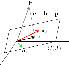
- $\mathbf b$ is not on the plane $C(A)$, but we project on it to get $\mathbf p$
- $\mathbf e$ is our projection error
Example
$\mathbb R^2$ Case
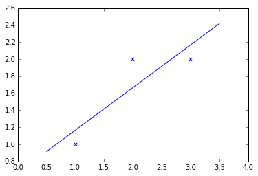
Suppose we have the following dataset:
- ${\cal D} = { (1,1), (2,2), (3,2) }$
so we have this system:
- $\left{\begin{array}{l}
x_0 + x_1 = 1\
x_0 + 2 x_1 = 2
x_0 + 2 x_1 = 3
\end{array}\right.$ - first column is always 1 because it’s our intercept term $x_0$, and $x_1$ is the slope
- the matrix form is $\begin{bmatrix}
1 & 1\
1 & 2\
1 & 3
\end{bmatrix} \begin{bmatrix} x_0 \ x_1 \end{bmatrix} = \begin{bmatrix} 1 \ 2 \ 2 \end{bmatrix}$ - no line goes through these points at once
- so we solve $A^T A \mathbf{\hat x} = A^T \mathbf b$
- $\begin{bmatrix}
1 & 1 & 1 \
1 & 2 & 3 \
\end{bmatrix} \begin{bmatrix}
1 & 1\
1 & 2\
1 & 3
\end{bmatrix} = \begin{bmatrix} 3 & 6\ 6 & 14
\end{bmatrix}$ - this system is invertible, so we solve it and get $\hat x_0 = 2/3, \hat x_1 = 1/2$
- thus the best line is $y = x_0 + x_1 t = 2/3 + 1/2 t$
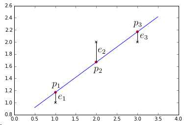
Is this indeed the best straight line through these points?
- we want to make the overall error as small as possible
- recall that $\mathbf e$ is our projection error - so we want to minimize it
- usually we minimize the square: $\min | \mathbf e |^2 = \min \big{ e_1^2 + e_2^2 + e_3^2 \big} $
- so we minimize this: $| \mathbf e |^2 = | A \mathbf x - \mathbf b |^2$
- we claim that the solution to $A^T A \mathbf{\hat x} = A^T \mathbf b$ minimizes $| A \mathbf x - \mathbf b |^2$
Let’s check if $\mathbf p \; \bot \; \mathbf e$
- $\mathbf{\hat x} = \begin{bmatrix} \hat x_0 \ \hat x_1 \end{bmatrix} = \begin{bmatrix} 2/3 \ 1/2 \end{bmatrix}$
- thus $\mathbf p = A \mathbf{ \hat x } = \begin{bmatrix} p_1 \ p_2 \ p_3 \end{bmatrix} = \begin{bmatrix} 7/6 \ 5/3 \ 13/6 \end{bmatrix}$
- $\mathbf p + \mathbf e = \mathbf b$, so $\mathbf e = \mathbf b - \mathbf p = \begin{bmatrix} 1 - 7/6 \ 2 - 5/3 \ 2 - 13/6 \end{bmatrix} = \begin{bmatrix} - 1/6 \ 2/3 \ -1/6 \end{bmatrix} $
- $\mathbf p \; \bot \; \mathbf e$ $\Rightarrow$ $\mathbf p^T \mathbf e = 0$.
- Check: $\begin{bmatrix} 7/6 & 5/3 & 13/6 \end{bmatrix} \begin{bmatrix} - 1/6 \ 2/3 \ -1/6 \end{bmatrix} = - 7/6 \cdot 1/6 + 5/3 \cdot 2/3 - 13/6 \cdot 1/6 = 0$
We can also verify that $\mathbf e \; \bot \; C(A)$
- let’s take one vector from $C(A)$, e.g. $\mathbf 1 = [1, 1, 1]^T \in C(A)$,
- $\mathbf e^T \cdot \mathbf 1 = -1/6 + 2/6 - 1/6 = 0$
Python code
```python import matplotlib.pylab as plt import numpy as np class Line: def __init__(self, slope, intercept): self.slope = slope self.intercept = intercept def calculate(self, x1): x2 = x1 * self.slope + self.intercept return x2 A = np.array([[1, 1], [1, 2], [1, 3]]) b = np.array([1, 2, 2]) x0, x1 = np.linalg.solve(A.T.dot(A), A.T.dot(b)) lsq = Line(x1, x0) 1. figure plt.scatter(A[:, 1], b, marker='x', color='black') points = np.array([0.5, 3.5]) plt.plot(points, lsq.calculate(points)) plt.scatter(A[:, 1], lsq.calculate(A[:, 1]), marker='o', color='red') plt.vlines(A[:, 1], b, lsq.calculate(A[:, 1])) plt.show() x = np.array([[x0], [x1]]) p = A.dot(x).reshape(-1) e = p - b print p.dot(e) ```Normal Equation vs Gradient Descent
- need to choose learning rate $\alpha$
- need to do many iterations
- works well with large $n$
Normal Equation:
- don’t need to choose $\alpha$
- don’t need to iterate - computed in one step
- slow if $n$ is large $(n \geqslant 10^4)$
- need to compute $(X^T X)^{-1}$ - very slow
- if $(X^T X)$ is not-invertible - we have problems
Additional
Orthogonalization
How to speed up computation of $(X^T X)^{-1}$?
- let’s make the columns of $X$ orthonormal: orthogonal to each other and of length 1
- we can do the QR Factorization and obtain matrix $X = QR$
- $Q^T Q = I$, and it simplifies the calculation a lot
- usual case: $\mathbf w = (X^T X)^{-1} X^T \mathbf y$
- with $X = QR$: $X^T X = R^T Q^T Q R = R^T R$
- so,
- $X^T X \mathbf w = X^T \mathbf y$
- $\cancel{R^T} R \mathbf w = \cancel{R^T} Q^T \mathbf y$
- $\mathbf w = R^{-1} Q^T \mathbf y$
- so it becomes much simpler: no need to invert $X^T X$ directly
Singular Value Decomposition
Let’s apply SVD to $X$:
- $X = U \Sigma V^T$, with $\text{dim } X = \text{dim } \Sigma$
- $\begin{align}
X \mathbf w - \mathbf y & = U \Sigma V^T \mathbf w - \mathbf y
& = U \Sigma V^T \mathbf w - U U^T \mathbf y
& = U (\Sigma V^T \mathbf w - U^T \mathbf y)
\end{align}$ - let $\mathbf v = V^T \mathbf w$ and $\mathbf z = U^T \mathbf y$
- then we have $U (\Sigma \mathbf v - \mathbf z)$
Orthogonal Matrices preserve the $L_2$-norm
- i.e. $| U \mathbf x | = | \mathbf x |$
- thus, $| \mathbf e | = | X \mathbf w - \mathbf y | = | U (\Sigma \mathbf v - \mathbf z) | = | \Sigma \mathbf v - \mathbf z|$.
- $| X \mathbf w - \mathbf y | = | \Sigma \mathbf v - \mathbf z|$
- $| \Sigma \mathbf v - \mathbf z|$ is easier to minimize than $| X \mathbf w - \mathbf y |$ So we reduced OLS Regression problem to a diagonal form
Minimization $| \Sigma \mathbf v - \mathbf z|$:
- $\text{diag}(\Sigma) = (\sigma_1, \ … \ , \sigma_r, 0, \ … \ , 0)$
- $\Sigma \mathbf v = \begin{bmatrix} \sigma_1 \mathbf v_1 \ \vdots \ \sigma_r \mathbf v_r \ 0 \ \vdots \ 0 \end{bmatrix}$ and therefore $\Sigma \mathbf v - \mathbf z = \begin{bmatrix} \sigma_1 v_1 - z_1 \ \vdots \ \sigma_r v_r - z_r \ -z_{r+1} \ \vdots \ -z_{m} \end{bmatrix}$
- since we minimizing it w.r.t. $\mathbf v$, only first $r$ components of $\Sigma \mathbf v - \mathbf z$ matter
- we can make these $\sigma_i v_i - z_i$ as small as possible by using $v_i = z_i / \sigma_i$
- so first $r$ components become 0, and the rest are $-c_i$, thus, $| \Sigma \mathbf v - \mathbf z |^2 = \sum\limits_{i = r+1}^m c_i^2$
- when $r = m$, $| \Sigma \mathbf v - \mathbf z | = 0$, but in this case there’s no need to Normal Equation
Summary:
- calculate $X = U \Sigma V^T$ and $\mathbf z = U^T \mathbf y$
- use $\mathbf v = \left( \cfrac{z_1}{\sigma_1}, \ … \ , \cfrac{z_r}{\sigma_r}, 0, \ … \ , 0 \right)$ to minimize $| \Sigma \mathbf v - \mathbf z|$
- since $\mathbf v = V^T \mathbf w$, we recover $\mathbf w$ as $\mathbf w = V \mathbf v$
- this gives solution $\mathbf w$ and residual error $| \Sigma \mathbf v - \mathbf z|$
Compact solution:
- if $X = U \Sigma V^T$, then $\mathbf w = V \Sigma^+ U^T \mathbf y$
- where $\Sigma^+ = \Big[ \text{diag}(\Sigma) \Big]^{-1}$ (invert only non-zero elements on the diagonal of $\Sigma$)
Regularization
We find $\mathbf w$ by calculating $\mathbf w = (X^T X + \lambda E^*)^{-1} \cdot X^T \cdot y$
- where $E^* \in \mathbb{R}^{(n + 1) \times (n + 1)}$
- and $E$ is almost identity matrix (1s on the main diagonal, the rest is 0s), except that the very first element is 0
- i.e. for $n = 2$ : $\left[\begin{matrix} 0 & 0 & 0 \ 0 & 1 & 0 \ 0 & 0 & 1 \ \end{matrix} \right]$
- because we don’t regularize for the bias input $x_{i0} = 1$
- $(X^T X + \lambda E^*)$ is always invertible
This is called Ridge Regression
- it can also be solved by both Normal Equation and Gradient Descent
Implementation
Implementation in Octave
pinv(X' * X) * X' * y
See Also
Sources
- Linear Algebra MIT 18.06 (OCW)
- Machine Learning (coursera)
- http://en.wikipedia.org/wiki/Linear_least_squares_%28mathematics%29
- http://www.seas.ucla.edu/~vandenbe/103/lectures/qr.pdf