Taylor Series

calculus functions series

Taylor Series

The idea behind Taylor Series is that any well-behaving Function (e.g. Continuous Functions) can be represented as a sum of Polynomials

Taylor and Maclaurin Series

A Taylor Series of $f(x)$ at $x=0$ is

$f(x) = \sum\limits_{k=0}^\infty \cfrac{f^{(k)}(0)}{k

}\, x^k$

- where $f^{(k)}(0)$ is $k$th Derivative of $f$ evaluated at $x=0$

- this kind of Taylor Series about $x = 0$ is sometimes called ‘‘Maclaurin Series’’

Taylor Series of $f(x)$ at $x = a$ is

$f(x) = \sum\limits_{k=0}^\infty \cfrac{f^{(k)}(a)}{k }\, (x - a)^k$ - this is the general form

Expansion as an Operator

Taylor Expansion is the process of turning a function to a Taylor Series

can think of it as an operator that takes a function and returns a Series

Examples

Famous expansions:

Exponential Function: $e^x = \sum\limits_{k=0}^{\infty} \frac{1}{k

} x^k$ of Exponential Function

- Trigonometric Functions:

- $\cos x = \sum\limits_{k=0}^\infty (-1)^k \cfrac{x^{2k}}{(2k)

}$ of Cosine

- $\sin x = \sum\limits_{k=0}^\infty (-1)^k \cfrac{x^{2k + 1}}{(2k + 1)

}$ of Sine

- it allows us to deal with these functions as with long sums of polynomials

Approximation

Taylor Series are used for approximations

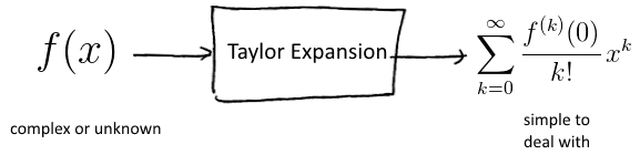
Exponential

as we add more terms, we are closer and closer to the function
(source: [http://www.wolframalpha.com/input/?i=e%5Ex+series])
order $n$ approximation is shown with $n$ dots

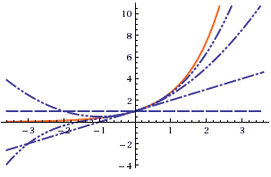
Trigonometric Functions:

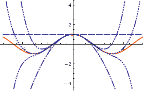(source: [http://www.wolframalpha.com/input/?i=cos+x+series])
(source: [http://www.wolframalpha.com/input/?i=sin+x+series])
by taking only polynomials of odd (even) powers, we get cosines or sines

Approximation near the expansion point 0:

Note that these approximations work best near 0
It’s clear from the sin/cos graphs - the more away from 0, need more terms

Computing Taylor Series

How to compute Taylor Series? There are several ways of doing it

Derivatives

This is the straightforward way:
use the definitions and compute all the Derivatives
if a function is complex, it may be hard

Substitution

Example: $\cfrac{1}{x}\, \sin (x^2)$

hard to take derivatives
but we know the expansion of $\sin x$, so
$\cfrac{1}{x}\, \sin (x^2) = \cfrac{1}{x}\, \left( (x^2) - \cfrac{1}{3| }\, (x^2)^3 + \cfrac{1}{5!}\, (x^2)^5 -\ … \right) =\ …$ | - $… \ = x - \cfrac{1}{3| }\, x^5 + \cfrac{1}{5!}\, x^9 -\ … = \sum\limits_{k=0}^\infty (-1)^k \cfrac{x^{4k + 1}}{(2k + 1)!}$ | |
Combination

$\cos^2 x = \cos x \cdot \cos x$
expand each one separately
$\cos x \cdot \cos x = \left(1 - \cfrac{1}{2| }\, x^2 + \cfrac{1}{4!}\, x^4 -\ … \right)\, \left( 1 - \cfrac{1}{2!}\, x^2 + \cfrac{1}{4!}\, x^4 -\ … \right) = \ …$ | - $… \ = 1\cdot 1 + 1\, \left(-\cfrac{1}{2| }\, x^2\right) + 1\, \left(\cfrac{1}{4!}\, x^4\right) + \ … \ - \cfrac{1}{2}\, x^2 \cdot 1 - \cfrac{1}{2}\, x^2 \left(-\cfrac{1}{2!}\, x^2\right) - \cfrac{1}{2}\, x^2 \left(\cfrac{1}{4!}\, x^4\right) - \ … \ = \ …$ | - $… \ = 1- x^2 +\cfrac{1}{3}\, x^4 - \cfrac{2}{45}\, x^6 + \ … $ |- since $\cos^2 x = 1 - \sin^2 x$, we also obtained the expansion of $\sin^2 x$| | |
Higher Order Terms

Instead of writing “…” can just say “HOT” meaning “Higher order terms”:

$e^x = 1 + x + \cfrac{1}{2}\, x^2 + \cfrac{1}{3

}\, x^3 + \text{HOT}$

- we mean that we don’t care what terms are there - it’s fine to consider just leading terms for some purposes

- it can simplify our calculations

For example:

$f(x) = 1 - 2x\, e^{\sin (x^2)}$
How can we Taylor Expand it?

$\sin (x^2) = x^2 - \cfrac{1}{3

}\, (x^2)^3 + \text{HOT} = x^2 - \cfrac{1}{3!}\, x^6 + \text{HOT}$

- $e^{\sin (x^2)} = 1 + \left( x^2 - \cfrac{1}{3

}\, x^6 + \text{HOT} \right) + \cfrac{1}{2!}\, \left( x^2 - \cfrac{1}{3!}\, x^6 + \text{HOT} \right)^2 + \cfrac{1}{3!}\, \left( x^2 + \text{HOT} \right)^3 + \text{HOT} = 1 + x^2 + \cfrac{1}{2}\, x^4 + \text{HOT}$

- so $f(x) = 1 - 2x\, e^{sin (x^2)} = 1 - 2x\, \left(1 + x^2 + \cfrac{1}{2}\, x^4 + \text{HOT} \right)$

To show what behavior HOTs have, we use Orders of Growth: the Big-O notation:

$e^x\, \cfrac{1}{1-x} = \big(1 + x + O(x^2)\big) \cdot \big(1 + x + O(x^2)\big) = \ …$
- $… \ = (1 + x)^2 + 2\, (1 + x)\, O(x) + \big( O(x^2)\big)^2 = 1 + 2x + O(x^2) + O(x^3) + O(x^4) = 1 + 2x + O(x^2)$

Convergence

Series = adding an infinite number of terms

it can be dangerous
Problem: not all functions can be expressed as sum of Polynomial Functions, i.e. as $f(x) = \sum c_k x^k$

for example, natural Logarithm:

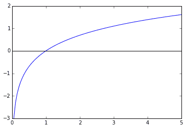
$\ln x$ is not even defined at $x=0$
polynomials are too simple to capture all the complexity of $\ln x$

Convergence Domain

Taylor Series has a ‘‘convergence domain’’ on which the series is well behaved

for many functions, e.g. $e^x$, $\sin x$, $\cos x$, $\sinh x$, etc, the domain is $\mathbb R = (-\infty, \infty)$

Within the domain of convergence you can do with series whatever you want:

rearrange terms
differentiate/integrate
combine

For example, $\ln (1 + x)$

$\ln (1 + x) = \int \cfrac{1}{1 + x}\, dx$
- $\cfrac{1}{1 + x}$ is Geometric Series, so
$\ln (1 + x) = \int \left(\sum\limits_{k=0}^\infty (-x)^k \right)\, dx = \ …$
- can rearrange integral and sum:
- $… \ = \sum\limits_{k=0}^\infty \left( \int (-x)^k \, dx \right) = \ …$
- $… \ = \sum\limits_{k=0}^\infty (-1)^k \cfrac{x^{k+1}}{k+ 1} + C = \ …$
$C = 0$ because $\ln 1 = 0$, so we have
- $\ln (1 + x) = \sum\limits_{k=1}^\infty (-1)^{k+1}\, \cfrac{x^k}{k} = x - \cfrac{1}{2}\, x^2 + \cfrac{1}{3}\, x^3 - \cfrac{1}{4}\, x^4 + \ …$
no factorials involved| | | ‘'’Convergence domain’’’:
we used Geometric Series here, so we must be in the domain of convergence of this series
which is $ x < 1$ - Taylor Series approximates well only on the domain of convergence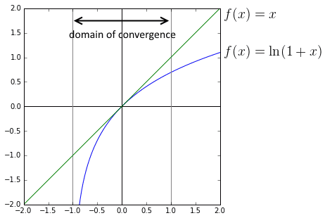
outside of the domain, we don’t get better approximation when we add more terms| | | Another example: $\arctan x$
$\arctan x = \int \cfrac{1}{1 + x^2}\, dx$
- we also have a Geometric Series here, with $-x^2$, so
$\arctan x = \int \cfrac{1}{1 + x^2}\, dx = \int \sum\limits_{k=0}^\infty (-x^2)^k \, dx = \ …$
- $… \ = \int \sum\limits_{k=0}^\infty (-1)^k x^{2k} \, dx = \sum\limits_{k=0}^\infty \left( \int (-1)^k x^{2k} \, dx \right) = \ …$
- $… \ = \sum\limits_{k=0}^\infty \cfrac{(-1)^k}{2k + 1}\, x^{2k + 1} + C$
$C = 0$ because $\arctan 0 = 0$
- so $\arctan x = x - \cfrac{1}{3}\, x^3 + \cfrac{1}{5}\, x^5 - \cfrac{1}{7}\, x^7 + \ …$
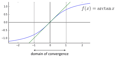
the domain of convergence is also $ x < 1$

Expansion Points

Maclaurin Series give good approximation at points near 0.
But what if we want to have good approximations at some other points?
In many applications 0 is not the most interesting point

Taylor Series of $f(x)$ at $x = a$ is

$f(x) = \sum\limits_{k=0}^\infty \cfrac{f^{(k)}(a)}{k| }\, (x - a)^k = f(a) + \cfrac{df}{dx}|{a} (x - a) + \cfrac{1}{2!}\, \cfrac{d^2f}{dx^2}|{a} (x - a)^2 + \cfrac{1}{3!}\, \cfrac{d^3f}{dx^3}|_{a} (x - a)^3 + \ …$ |- this is polynomial in $(x - a)$ instead of just $x$ |
Approximation

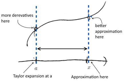
The bigger $

a - x

$ is, the more high-order terms we need to have good approximation

- Taylor Series converge only within the domain of convergence - so need to stay within the domain

Example:

estimate $\sqrt{10}$
$\sqrt{x}$ expanded at $x = a$ is $\sqrt{x} = \sqrt{a} + \cfrac{1}{2\, \sqrt{a}}\, (x - a) - \cfrac{1}{8\, \sqrt{a^3}}\, (x - a)^2 + \text{HOT}$

let’s approximate it at $a = 1$:

$\sqrt{x} = 1 + \cfrac{1}{2}\, (x - 1) - \cfrac{1}{8}\, (x - 1)^2 + \text{HOT}$
for $x = 10$, we get $\approx -4.122$

bad approximation

$a = 1$ is far from $x = 10$, so need more derivatives to approximate better

- let’s consider $a = 9$ ($\sqrt{9} = 3$)

- $\sqrt{x} = 3 + \cfrac{1}{6}\, (x - 9) - \cfrac{1}{216}\, (x - 9)^2 \approx -4.122$

for $x = 10$ we get $3 + 1/6 - 1/216 \approx 3.1620$ (real is $3.1623$)

quite close

- so it’s important to select $a$ which is close to the value $x$ where you want to approximate $f(x)$

Taylor Expansion via Decomposition

Be careful with expansion points when doing Taylor Expansion via decomposition Expand about the correct value| | |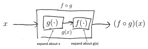

For example, compute expansion for $e^{\cos x}$ about $x = 0$

we have: $0 \to \cos (\cdot) \to e^{(\cdot)} \to$
first, we expand about 0
but for $e$, we don’t expand about 0 - we expand about $\cos 0 = 1$| |- $\cos x = 1 - \cfrac{1}{2| }\, x^2 + \cfrac{1}{4!}\, x^4 - \ …$ |- $e^u = e + e\, (u - 1) + \cfrac{1}{2| }\, e\, (u - 1)^2 + \ …$ | |
Sources
Calculus: Single Variable (coursera)

✏️ Edit on GitHub

Taylor Series

Taylor Series

Taylor and Maclaurin Series

Expansion as an Operator

Examples

Approximation

Computing Taylor Series

Derivatives

Substitution

Combination

Higher Order Terms

Convergence

Convergence Domain

Expansion Points

Approximation

Taylor Expansion via Decomposition

Sources