Learning Curves
This is a good technique (a part of Machine Learning Diagnosis)
- to sanity-check a model
- to improve performance
A ‘‘learning curve’’ is a plot where we have two functions of $m$ ($m$ is a set size):
- training set error $J_{\text{train}}(\theta)$,
- the cross-validation error $J_{\text{cv}}(\theta)$
We can artificially reduce our training set size.
- We start from $m = 1$, then $m = 2$ and so on
So suppose we have the following model:
- $h_{\theta}(x) = \theta_0 + \theta_1 x + \theta_2 x^2$

- for each $m$ we calculate $J_{\text{train}}(\theta)$ and $J_{\text{cv}}(\theta)$ and plot the values
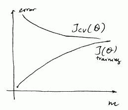
- This is the learning curve of the model
Diagnose High Bias (Underfitting)
- Suppose we want to fit a straight line to out data:
- $h_{\theta}(x) = \theta_0 + \theta_1 x$
As $m$ increases we have pretty same line:
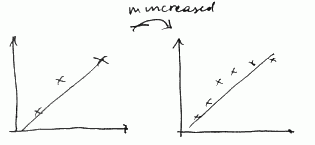
If we draw the learning curves, we’ll have
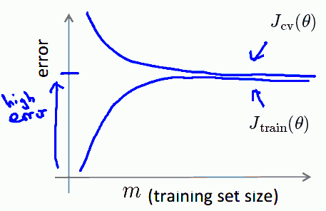
So we see that
- as $m$ grows $J_{\text{cv}}(\theta) \to J_{\text{train}}(\theta)$
- and both errors are high
$\Rightarrow$ If learning algorithm is suffering from high bias, getting more examples will not help
Diagnose High Variance (Overfitting)
- Now suppose we have a model with polynomial of very high order:
- $h_{\theta}(x) = \theta_0 + \theta_1 x + \theta_2 x^2 + … + \theta_{100} x^{100}$
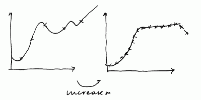
- at the beginning we very much overfit
- as we increase $m$, we still able to fit the data well
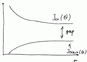
So we can see that as $m$ increases,
- $J_{\text{train}}(\theta)$ increases (we have more and more data - so it’s harder and harder to fit $h_{\theta}(x)$), but it increases very slowly
- on the other hand, $J_{\text{cv}}(\theta)$ decreases, but also very very slow
- and there’s a huge gap between these 2
- to fill that gap we need many many more training examples
$\Rightarrow$ if a learning algorithm is suffering from high variance (i.e. it overfits), getting more data is likely to help