Neural Networks

machine-learning

Motivation

Suppose we have a large number of features and a complex structure of data
For Logistic Regression we would probably need to fit a very high-order polynomial

Say we have 100 features ($n = 100$) and we want to fit, a multiplication of each pair of features

i.e. we will have $x_1^2, x_1 x_2, …, x_1 x_{100}, … x_2^2, x_2 x_3, …, $
this gives us $\approx$ 5000 features (it grows as $O(n)$)

for combinations of triples we’ll have $\approx$ 170 000 features

Next, suppose we have a computer vision problem: car detection

we show it cars, then show it not cars, and then test
Say we have 50 x 50 pixels image, 2500 pixels in total (7500 if RGB).
If we want to fit polynomials, the number of features is too huge to do this| | | So using Logistic Regression is certainly not a good way to handle lots of features, and here Neural Networks can help

Neural Networks

This technique is based on how our brain works - it tries to mimic its behavior.

Model Representation

A NN model is built from many ‘‘neurons’’ - cells in the brain.
the neuron, called ‘‘activation unit’’, takes features as input
A network consists of many activation units

Sigmoid Activation Unit

the simplest activation unit is a Logistic Regression
i.e. it is equivalent to Logistic Regression model

it’s called ‘‘sigmoid (logistic) activation function’’:

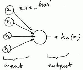
Bias unit

$x_0$ is a bias unit, $x_0 = 1$ always
$x_0$ may be omitted from a picture, but it’s usually assumed in these cases

Weights

arrows are “input wires”
so this unit takes $x = [x_0, x_1, x_2, x_3]^T$,
and the wires are out parameters $\theta = [\theta_0, \theta_1, \theta_2, \theta_3]^T$ - their are called ‘‘weights’’

Result

it applies the sigmoid function to the input, and as the result, it returns
$h_{\theta} = g(\theta^T x) = \cfrac{1}{1 + e^{-\theta^T x}}$

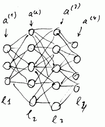
Neural Network Model

Let’s have a look at an actual neural network

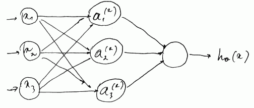
A NN model is a network of many sigmoid activation units, organized in ‘‘layers’’
- where the next layer’s input is the current layer’s output
the first layer is ‘‘input layer’’, called $x$ - it takes our feature vector $x = [x_1, …, x_n]^T$
the last layer (3rd on the picture) is an output layer, it gives us the final result
all layers in between are called ‘‘hidden layers ‘’
(note that bias units $x_0$ and $a_0^{(2)}$ are omitted from the picture, but they are there)

Mathematical Representation

We’ll have the following notation:

$a_i^{(j)}$ is an ‘‘activation of unit $i$ in layer $j$’’
$\theta^{(j)}$ - matrix of ‘‘weights’’ that control mapping from layer $j$ to $j + 1$ (i.e. $\theta_1$ is the parameters of the 2nd layer and so on)
Neural Networks are parametrized by $\theta$s

Mathematical representation of a neural network is (where $g$ is the sigmoid function)

$a_1^{(2)} = g(\theta_{10}^{(1)} x_0 + \theta_{11}^{(1)} x_1 + \theta_{12}^{(1)} x_2 + \theta_{13}^{(1)} x_3)$
$a_2^{(2)} = g(\theta_{20}^{(1)} x_0 + \theta_{21}^{(1)} x_1 + \theta_{22}^{(1)} x_2 + \theta_{23}^{(1)} x_3)$
$a_3^{(2)} = g(\theta_{30}^{(1)} x_0 + \theta_{31}^{(1)} x_1 + \theta_{32}^{(1)} x_2 + \theta_{33}^{(1)} x_3)$
and $h_{\theta}(x) = a_1^{(3)} = g(\theta_{10}^{(2)} a_0^{(2)} + \theta_{11}^{(2)} a_1^{(2)} + \theta_{12}^{(2)} a_2^{(2)} + \theta_{13}^{(2)} a_3^{(2)})$

so we have

3 input units $x_1, x_2, x_3$ (plus bias $x_0 = 1$)
3 hidden units in 1 hidden layer $a_1^{(2)}, a_2^{(2)}, a_3^{(2)}$ in layer 2 (plus bias $a_0^{(2)} = 1$)

Dimension of $\theta$

In this example the dimension of $\theta^{(1)}$ is $\theta^{(1)} \in \mathbb{R}^{3 \times 4}$

General rule

if a network has $s_j$ units in layer $j$ and $s_{j + 1}$ units in layer $j + 1$ , then
$\theta^{(i)} \in \mathbb{R}^{s_{j + 1} \times (s_{j} + 1)}$ (i.e. it has dimension $s_{j + 1} \times (s_{j} + 1)$)

Forward Propagation

Vectorized Form

For the first step we have

$a_1^{(2)} = g(z_1^{(2)})$ where $z_1^{(2)} = \theta_{10}^{(1)} x_0 + \theta_{11}^{(1)} x_1 + \theta_{12}^{(1)} x_2 + \theta_{13}^{(1)} x_3$
$a_2^{(2)} = g(z_2^{(2)})$, and
$a_3^{(2)} = g(z_3^{(2)})$
($z_1^{(2)}, z_2^{(2)}, z_3^{(2)}$ - are ‘‘linear combinations’’ of $x_1, x_2, x_3$)

So we have 3 vectors

$\theta^{(0)} = [\theta_0^{(0)}, \theta_1^{(0)}, \theta_2^{(0)}, \theta_3^{(0)}]^T$,
$x = [x_0, x_1, x_2, x_3]^T$,
$z^{(2)} = [z_1^{(2)}, z_2^{(2)}, z_3^{(2)}]^T$

And can rewrite the first step in a vectorized form:

instead of $z_1^{(2)} = \theta_{10}^{(1)} x_0 + \theta_{11}^{(1)} x_1 + \theta_{12}^{(1)} x_2 + \theta_{13}^{(1)} x_3$, we write $z_1^{(2)} = \theta_1^{(1)} \cdot x$

Algorithm

1st step
- $z^{(2)} = \theta^{(1)} \cdot x = \theta^{(1)} \cdot a^{(1)}$ and
- $a^{(2)} = g(z^{(2)}) \in \mathbb{R}^3$
next step
- we add $a_0^{(2)} = 1$, so $a^{(2)} = [1, a_1^{(2)}, a_2^{(2)}, a_3^{(2)}]^T \in \mathbb{R}^{4}$
- and calculate $z^{(3)} = \theta^{(2)} \cdot a^{(2)}$
finally
- $h_{\theta}(x) = a^{(3)} = g(z^{(3)})$

This process is called ‘‘forward propagation’’

What’s going on?

Let’s have a look at the 2nd and 3rd layers of our NN

$h_{\theta} = g((\theta^{(2)})^T \cdot a^{(2)})$, and $a^{(2)}$ is given by the 2nd level units
so it’s doing a logistic regression, but it uses $a^{(2)} = [a_0^{(2)} … a_3^{(2)}]$ for features (instead of $x$s)
and features $a^{(2)} = [a_0^{(2)} … a_3^{(2)}]$ are themselves learned by the previous layer
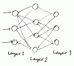
We can create NNs with as many layers as we want
The way the neurons are connected is called ‘‘architecture’’

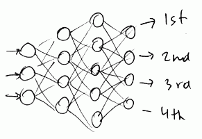
Multi-class Classification

What to do if we what to use it for multi-class classification?

We can have multiple output units (similar to One-vs-All Classification) So we want
$h_{\theta}(x) \approx \left[\begin{matrix} 1 \ 0 \ 0 \ 0\end{matrix} \right]$ if an item belongs to 1st category
$h_{\theta}(x) \approx \left[\begin{matrix} 0 \ 1 \ 0 \ 0\end{matrix} \right]$ if it belongs to 2nd category
and so on

For training set ${(x^{(i)}, y^{(i)})}$

we turn $y$ into one of $\left{ \left[\begin{matrix} 1 \ 0 \ 0 \ 0\end{matrix} \right], \left[\begin{matrix} 0 \ 1 \ 0 \ 0\end{matrix} \right], \left[\begin{matrix} 0 \ 0 \ 1 \ 0\end{matrix} \right], \left[\begin{matrix} 0 \ 0 \ 0 \ 1\end{matrix} \right] \right}$ - instead of $y \in {1, 2, 3, 4}$,
so, when training, we would like to have $h_{\theta}(x^{(i)}) \approx y^{(i)} \in \mathbb{R}^4$
then we select the class with highest $h_{\theta}^{(i)}(x^{(i)})$, as in One-vs-All Classification

Cost Function

Suppose we have $m$ training examples ${(x^{(i)}, y^{(i)})}$

$L$ - total number of layers in network
$S_l$ - # of units (without bias) in layer $l$
$K = S_L$ - number of units the output layer, i.e. the network classifies $K$ classes

output $h_{\theta}(x) \in \mathbb{R}^{K}$

For example,

$L = 3$
$S_1 = 3, S_2 = 4, K = S_3 = 3$

For Logistic Regression with Regularization we have the following cost function:

\[J(\theta) = -\cfrac{1}{m} \sum \Big[ y^{(i)} \log h_{\theta}(x^{(i)}) + (1 - y^{(i)}) \log (1 - h_{\theta}(x^{(i)})) \Big] + \cfrac{\lambda}{2m} \sum_{j = 1}^{n} \theta_j^2\]

In neural networks

$h_{\theta}(x) \in \mathbb{R}^K$
let $h_{\theta}(x)_i$ - be $i$th output

So we have

\[J(\theta) = -\cfrac{1}{m} \sum_{i = 1}^{m} \sum_{k = 1}^{K} \Big[ y_k^{(i)} \log h_{\theta}(x^{(i)})_k + (1 - y_k^{(i)}) \log (1 - h_{\theta}(x^{(i)})_k ) \Big] + \cfrac{\lambda}{2m} \sum_{l = 1}^{L - 1} \sum_{i = 1}^{S_l} \sum_{j = 1}^{S_{l + 1}} (\theta_{ji}^{l})^2\]

here we also don’t regularize bias inputs

Back Propagation

we need to find such $\theta$ that $J(\theta)$ is minimal
for that we can use Gradient Descent or other advanced optimization techniques
for GD we need to compute partial derivative $\cfrac{\partial}{\partial \theta_{ij}^{(l)}} J(\theta)$ with respect to each $\theta_{ij}^{(l)}$

'’Back Propagation’’ is a technique for calculating partial derivatives in neural networks

suppose we have a training example $(x, y)$

To compute cost $J(\theta)$ we use Forward Propagation (vectorized)

$a^{(1)} = x$
$z^{(2)} = \theta^{(1)} \cdot a^{(1)}$
$a^{(2)} = g(z^{(2)})$ (plus adding $a_0^{(2)} = 1$)
$z^{(3)} = \theta^{(2)} \cdot a^{(2)}$
$a^{(3)} = g(z^{(3)})$ (plus adding $a_0^{(3)} = 1$)
$z^{(4)} = \theta^{(3)} \cdot a^{(4)}$
$a^{(4)} = g(z^{(4)})$ (plus adding $a_0^{4)} = 1$)

Back Propagation Overview

To compute derivatives we use Back Propagation

let $\delta_j^{(l)} $be “error” of node $j$ in layer $i$ (for $a_j^{(l)}$)
for each output unit we compute
- $\delta_k^{(L)} = a_j^{(L)} - y_j = h_{\theta}(x)_j - y_j$
- or, vectorized:
: $\delta^{(L)} = a^{(L)} - y$

next, we compute $\delta$ for all earlier layers

$\delta^{(3)} = (\theta^{(3)})^T \cdot \delta^{(4)} * g’(z^{(3)})$
where
- $*$ - element-wise product
- $g’(z^{(3)})$ - derivative of function $g$ in $z^{(3)}$
- $g’(z^{(3)}) = a^{(3)} * (1 - a^{(3)})$
$\delta^{(2)} = (\theta^{(2)})T \cdot \delta^{(3)} .* g’(z^{(2)})$
We don’t compute anything for the first layer - it’s the input layer, and there can be no errors

Our partial derivative is

$\cfrac{\partial}{\partial \theta_{ij}^{(l)}} J(\theta) = a_j^{(l)} \cdot \delta_i^{(l + 1)}$
(here we ignore regularization parameter $\lambda$ - i.e. we assume no regularization at the moment)

Back Propagation Algorithm

We have training set ${(x^{(i)}, y^{(i)}}$ with $m$ training examples

Set $\Delta_{ij}^{(l)} \leftarrow 0$ for all $l$, $i$, $j$ (it’s used to compute$ \cfrac{\partial}{\partial \theta_{ij}^{(l)}} J(\theta)$ )

For each ${(x^{(i)}, y^{(i)}}$:

set $a^{(1)} = x^{(i)}$
perform Forward Propagation to compute $a^{(l)}$ for $l = 2, 3, …, L$
perform Back Propagation
- Using $y^{(i)}$ compute $\delta^{(L)} = a^{(L)} - y^{(i)}$
- Then compute
  - all $\delta^{(L - 1)}, \delta^{(L - 2)}, …, \delta^{(2)}$
  - Set $\Delta_{ij}^{(l)} \leftarrow \Delta_{ij}^{(l)} + a_j^{(l)} \delta_i^{(l + 1)} $
  - or, vectorized:
- : $\Delta^{(l)} \leftarrow \Delta^{(l)} + \delta^{(l + 1)} (a^{(l)})^T$
Then we calculate
- $D_{ij}^{(l)} \leftarrow \cfrac{1}{m} \delta_{ij}^{(l)} + \lambda \theta_{ij}^{(l)}$ if $j \ne 0$
- $D_{ij}^{(l)} \leftarrow \cfrac{1}{m} \delta_{ij}^{(l)}$ if $j = 0$
That value can we used for GD:

$\cfrac{\partial}{\partial \theta_{ij}^{(l)}} = D_{ij}^{(l)}$

To sum up, for each training example we

propagate forward using $x$
we back-propagate using $y$
add up all error units (for each $\theta$) into matrix $\Delta$

Intuition

Say we have a single training example $(x, y)$ and 1 output unit and we ignore regularization

$\text{cost}(x, y) = y \log h_{\theta}(x) + (1 - y) \log h_{\theta}(x)$

it calculates how well is the network doing for that training example - how close it is to $y$?
$\delta_j^{(l)}$ = “error” of cost for $a_j^{(l)}$ (unit $j$ in layer $l$)

formally,

$\delta_j^{(l)} = \cfrac{\partial}{\partial z_j^{(l)}} \text{cost}(x, y)$
it’s a partial derivative with respect to $z_j^{(l)}$
they are measures how much we would like to change the NN weights in order
- to affect intermediate values $z^{(2)}, z^{(3)}, …,$
- and the final output $z^{(4)}$,
- and therefore, overall cost

Numerical Gradient Checking

Implementing back-propagation can be hard and bug-prone, but we can perform Numerical Gradient Checking to test our implementation

suppose $\theta \in \mathbb{R}$

We can estimate real slope of the derivative by calculating $J(\theta + \epsilon) - J(\theta - \epsilon)$ for small $\epsilon$
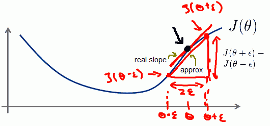
$\cfrac{d}{d \theta} J(\theta) \approx \cfrac{J(\theta + \epsilon) - J(\theta - \epsilon)}{2\epsilon}$
And that will give us a numerical estimate of the gradient and that point

when $\theta \in \mathbb{R}^n$

for partial derivative with respect to each $\theta_i$ we calculate
$\cfrac{\partial}{\partial \theta_1} J(\theta) \approx \cfrac{J(\theta_1 + \epsilon, \theta_2, …, \theta_n) - J(\theta_1 - \epsilon, \theta_2, …, \theta_n)}{2\epsilon}$
$\cfrac{\partial}{\partial \theta_2} J(\theta) \approx \cfrac{J(\theta_1, \theta_2 + \epsilon, …, \theta_n) - J(\theta_1, \theta_2 - \epsilon, …, \theta_n)}{2\epsilon}$
…
$\cfrac{\partial}{\partial \theta_2} J(\theta) \approx \cfrac{J(\theta_1, \theta_2, …, \theta_n + \epsilon) - J(\theta_1, \theta_2, …, \theta_n - \epsilon)}{2\epsilon}$
i.e. we add and subtract only values for $\theta_i$ we calculate derivative for
this gives us a way to numerically estimate all partial derivatives
and then we check if this numerical estimate $\approx$ the derivative from back propagation

Implementation Notes

To implement Back Propagation use the following approach:

Implement back propagation to compute $D^{(1)}, D^{(2)}, …$
Implement numerical gradient check to compute approximations of partial derivatives
Make sure they have similar values
Turn off gradient checking, use only back propagation for learning (it’s much more computationally efficient)

Random Initialization

We need to have initial values for $\theta$
In Logistic Regression we used $\theta = [0, 0, …, 0]^T$
It won’t work for NNs

Suppose we set all $\theta_{ij}^{(l)}$ to 0

Then we’ll have same values for $a_1^{(2)} = a_2^{(2)} = … = a_{s_2}^{(2)}$ and same for $\delta^{(2)}$

(after each update, parameters corresponding to inputs are identical, and all hidden units will compute the same value)
And therefore, all partial derivatives will also we equal
This is called ‘‘the problem of symmetric weights’’

We can break the symmetry with random initialization

so, initialize each $\theta_{ij}^{(l)}$ with random value from $[-\epsilon; \epsilon]$:
$\theta_{ij}^{(l)} \leftarrow_{r} [-\epsilon; \epsilon]$

Implementation

Algorithm

Randomly initialize weights $\theta$
Implement forward propagation to get $h_{\theta}(x^{(i)})$ for any $x^{(i)}$
Implement code to compute cost function $J(\theta)$
Implement back propagation to compute partial derivatives $\cfrac{\partial}{\partial \theta_{ij}^{(l)}} J(\theta)$
Use gradient checking to compare numerical estimations of partial derivatives vs values from back propagation
Use Gradient Descent or another optimization technique to minimize $J(\theta)$

’'’NB’’’: $J(\theta)$ in non-convex and can get stuck in local minimum - but usually it’s not a problem

Octave

Cost Function (both forward propagation and back propagation)
One-vs-All Prediction for NN
Numerical Gradient Check

Sources

Machine Learning (coursera)

✏️ Edit on GitHub

Neural Networks

Motivation

Neural Networks

Model Representation

Sigmoid Activation Unit

Neural Network Model

Mathematical Representation

Dimension of $\theta$

Forward Propagation

Vectorized Form

Algorithm

What’s going on?

Multi-class Classification

Cost Function

Back Propagation

Back Propagation Overview

Back Propagation Algorithm

Intuition

Numerical Gradient Checking

Implementation Notes

Random Initialization

Implementation

Algorithm

Octave

See also

Sources