Regularization
- '’Regularization’’ is a technique used to address overfitting
- Main idea of regularization is to keep all the features, but reduce magnitude of parameters $\theta$
- It works well when we have a lot of features, each of which contributes a bit to predicting $y$
Penalization
- Suppose we want to fit $\theta_0 + \theta_1 x_1 + \theta_2 x_2 + \theta_3 x_3 + \theta_4 x_4$
- We want to penalize $\theta_3$ and $\theta_4$ - and make them small
-
- we modify out cost function $J$:
- $J(\theta) = \cfrac{1}{m} \left[ \sum_{i=1}^{m} \text{cost}(h_{\theta}(x^{(i)}), y^{(i)}) + 1000 \cdot \theta_3^2 + 1000 \cdot \theta_4^2 \right]$
- where $1000 \cdot \theta_3^2$ and $1000 \cdot \theta_4^2$ - ‘‘penalty’’ for using $\theta_3$ and $\theta_4$ respectively
- As a result, we’ll have $\theta_3 \approx 0$ and $\theta_4 \approx 0$
So, ‘‘regularization’’ ensures that values for $\theta_1 … \theta_n$ are small
- it makes the hypotheses simple
- and less prone to overfitting
Cost Function
- we have features $x_1, …, x_m$ - they may be polynomials
- and parameters $\theta_0, \theta_1, …, \theta_m$
We don’t know which parameter to penalize.
Here is our cost function $J$ with regularization:
- $J(\theta) = \cfrac{1}{m} \left[ \sum_{i=1}^{m} \text{cost}(h_{\theta}(x^{(i)}), y^{(i)}) + \lambda \sum_{j = 1}^{n} \theta_j^2 \right]$
- In the cost function we include the penalty for all $\theta$s
- we typically don’t penalize $\theta_0$, only $\theta_1, …, \theta_n$
- $\lambda$ is called ‘‘regularization parameter’’
Regularization Parameter $\lambda$
When we find the optimum for our cost function $J$ we have two goals:
- we would like to fit the training data well
- 1st term of the expression reflects that:
- $\sum_{i=1}^{m} (\text{cost}(h_{\theta}(x^{(i)})), y^{(i)})$
- we want to keep the parameters small
- 2nd term ensures that:
- $\lambda \sum_{j = 1}^{n} \theta_j^2$
$\lambda$ is the paramenter that controls the trade-off between these two goals
- We need to choose $\lambda$ carefully
- large $\lambda$ will lead to underfitting (we’ll end up with $h_{\theta}(x) \approx \theta_0$ )
Say we want to fit $h_{\theta}(x) = \theta_0 + \theta_1 x + … + \theta_4 x^4$
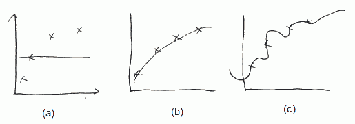
- (a) If $\lambda$ if large (say $\lambda = 10000$), all $\theta$ are penalized and $\theta_1 \approx \theta_2 \approx … \approx 0$, $h_{\theta}(x) \approx \theta_0$
- (b) if $\lambda$ is intermediate, we fit well
- (c) if $\lambda$ is small (close to 0) we fit too well, i.e. we overfit
To find the best value for this parameter, Model Selection techniques can be used. For example, Cross-Validation
Usage
Regularized Linear Regression
Gradient Descent
When we use Gradient Descent (or other optimization technique), we have the following algorithm:
- repeat:
- for all $j$
- $\theta_j = \theta_j - \cfrac{\partial}{\partial \theta_j} J(\theta)$
Because we have changed the $J(\theta)$ by adding the regularization term, we need to change the partial derivatives of $J(\theta)$. So the algorithm now looks as follows:
- repeat
- $\theta_0 = \theta_0 - \cfrac{\alpha}{m} \sum (h_{\theta}(x^{(i)}) - y^{(i)}) x_0^{(i)}$ // no change for $\theta_0$
- $\theta_j = \theta_j - \alpha \left[ \cfrac{1}{m} \sum (h_{\theta}(x^{(i)}) - y^{(i)}) x_0^{(i)} + \cfrac{\lambda}{m} \theta_j \right]$
Or we can rewrite the last one as: $\theta_j = \theta_j \left(1 - \alpha \cfrac{\lambda}{m} \right) - \cfrac{\alpha}{m} \sum (h_{\theta}(x^{(i)}) - y^{(i)}) x_0^{(i)}$
Normal Equation
We have the following input:
- $X = \left[\begin{matrix} … (x^{(1)})^T … \ … \ … (x^{(m)})^T … \end{matrix} \right] \in \mathbb{R}^{m \times (n + 1)}$
- $y = \left[\begin{matrix} y_1 \ \vdots \ y_m \end{matrix} \right] \in \mathbb{R}^{m}$
We find $\theta$ by calculating $\theta = (X^T X + \lambda E^*)^{-1} \cdot X^T \cdot y$
- where $E^* \in \mathbb{R}^{(n + 1) \times (n + 1)}$
- and $E$ is almost identity matrix (1s on the main diagonal, the rest is 0s), except that the very first element is 0
- i.e. for $n = 2$ : $\left[\begin{matrix} 0 & 0 & 0 \ 0 & 1 & 0 \ 0 & 0 & 1 \ \end{matrix} \right]$
- $(X^T X + \lambda E^*)$ is always invertible
Regularized Logistic Regression
-
- Old cost function for Logistic Regression (without regularization) is:
- $J_{\text{old}}(\theta) = - \cfrac{1}{m} \sum \left[ y \cdot \log(h_{\theta}(x)) + (1 - y) \cdot \log(1 - h_{\theta}(x)) \right]$
-
- We need to modify it to penalize $\theta_1, …, \theta_n$:
- $J(\theta) = J_{\text{old}}(\theta) + \cfrac{\lambda}{2m} \sum_{j = 1}^{n} \theta_j^2$
Similarly, for Gradient Descent we have
- repeat
- $\theta_0 = \theta_0 - \cfrac{\alpha}{m} \sum (h_{\theta}(x^{(i)}) - y^{(i)}) x_0^{(i)}$ // no change for $\theta_0$
- $\theta_j = \theta_j - \alpha \left[ \cfrac{1}{m} \sum (h_{\theta}(x^{(i)}) - y^{(i)}) x_0^{(i)} + \cfrac{\lambda}{m} \theta_j \right]$