OLS Regression

linear-algebra machine-learning regression statistics

Ordinary Least Squares Regression

This is a technique for computing coefficients for Multivariate Linear Regression.
the solution is obtained via minimizing the squared error, therefore it’s called ‘‘Linear Least Squares’’
two solutions: Normal Equation and Gradient Descent
this is the the typical way of solving the Multivariate Linear Regression, therefore it’s often called ‘'’OLS Regression’’’

Suppose we have

$m$ training examples $(\mathbf x_i, y_i)$
$n$ features, $\mathbf x_i = \big[x_{i1}, \ … \ , x_{in} \big]^T \in \mathbb{R}^n$
We can put all such $\mathbf x_i$ as rows of a matrix $X$ (sometimes called a ‘‘design matrix’’)
$X = \begin{bmatrix}
\ \mathbf x_1^T - \ \vdots \
\ \mathbf x_m^T - \ \end{bmatrix} = \begin{bmatrix} x_{11} & \cdots & x_{1n} \ & \ddots & \ x_{m1} & \cdots & x_{mn} \ \end{bmatrix}$
the observed values: $\mathbf y = \begin{bmatrix} y_1 \ \vdots \ y_m \end{bmatrix} \in \mathbb{R}^{m}$
Thus, we expressed our problem in the matrix form: $X \mathbf w = \mathbf y$
Note that there’s usually additional feature $x_{i0} = 1$ - the slope,
- so $\mathbf x_i \in \mathbb{R}^{n+1}$ and $X = \begin{bmatrix}
\ \mathbf x_1^T - \
\ \mathbf x_2^T - \ \vdots \
\ \mathbf x_m^T - \ \end{bmatrix} = \begin{bmatrix} x_{10} & x_{11} & \cdots & x_{1n} \ x_{20} & x_{21} & \cdots & x_{2n} \ & & \ddots & \ x_{m0} & x_{m1} & \cdots & x_{mn} \ \end{bmatrix} \in \mathbb R^{m \times n + 1}$

Thus we have a system

$X \mathbf w = \mathbf y$
how do we solve it, and if there’s no solution, how do we find the best possible $\mathbf w$?

There’s no solution to the system, so we try to fit the data as good as possible

Let $\mathbf w$ be the best fit solution to $X \mathbf w \approx \mathbf y$
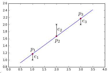
we’ll try to minimize the error $\mathbf e = \mathbf y - X \mathbf w$ (also called residuals)
we take the square of this error, so the objective is
$J(\mathbf w) = | \mathbf e |^2 = | \mathbf y - X \mathbf w |^2$

The solution:

From the Linear Algebra point of view:

we need to solve $X \mathbf w = \mathbf y$
if $\mathbf y \not \in C(X)$ (Column Space) then there’s no solution
How to solve it approximately? Project on $C(A)$ - again, it gives us the Normal Equation: $X^T X \mathbf w = X^T \mathbf y$

Alternatively, we can use Gradient Descent:

objective is $J(\mathbf w) = | \mathbf y - X \mathbf w |^2$

- the derivative w.r.t. $\mathbf w$ is $\cfrac{\partial J(\mathbf w)}{\partial \mathbf w} = 2 X^T X \mathbf w - 2 X^T \mathbf y$

so the update rule is $\mathbf w \leftarrow \mathbf w - \alpha 2 (X^T X \mathbf w - X^T \mathbf y)$
where $\alpha$ is the learning rate

Suppose we have the following dataset:

${\cal D} = { (1,1), (2,2), (3,2) }$
the matrix form is $\begin{bmatrix} 1 & 1\ 1 & 2\ 1 & 3
\end{bmatrix} \begin{bmatrix} w_0 \ w_1 \end{bmatrix} = \begin{bmatrix} 1 \ 2 \ 2 \end{bmatrix}$
no line goes through these points at once
so we solve $X^T X \mathbf{\hat w} = X^T \mathbf y$
$\begin{bmatrix} 1 & 1 & 1 \ 1 & 2 & 3 \ \end{bmatrix} \begin{bmatrix} 1 & 1\ 1 & 2\ 1 & 3
\end{bmatrix} = \begin{bmatrix} 3 & 6\ 6 & 14
\end{bmatrix}$
this system is invertible, so we solve it and get $\hat w_0 = 2/3, \hat w_1 = 1/2$
thus the best line is $h(t) = w_0 + w_1 t = 2/3 + 1/2 t$