$\require{cancel}$
Projections
Suppose we have an $n$-dimensional subspace that we want to project on
- what do we do?
Two-Dimensional Case: Motivation and Intuition
Suppose we have two vectors $\mathbf a$ and $\mathbf b$
- we want to ‘‘project’’ $\mathbf b$ to $\mathbf a$: find a point on $\mathbf a$ that is closest to $\mathbf b$

- let $\mathbf e$ be the vector from $\mathbf b$ to $\mathbf a$ - it’s our ‘‘projection error’’ - how much we’re wrong about it
- let $\mathbf p$ be the projection of $\mathbf b$ to $\mathbf a$
- $\mathbf e = \mathbf b - \mathbf p$
Trigonometry

- (Triangle method of subtraction)
Can use trigonometry to do it
-
magnitude is $| \mathbf e | = \sqrt{ | \mathbf p | ^2 - | \mathbf b |^2 - 2 \cdot | \mathbf p | \cdot | \mathbf b | }$ - so we want to find such $\mathbf p$ that minimizes the magnitude of $\mathbf e$ - it’s nasty, we don’t want to deal with it
- alternatively can use Linear Algebra for that
Linear Algebra
The ‘‘closest’’ - means that $\mathbf e$ must be as small as possible
- it’s possible when $\mathbf e \; \bot \; \mathbf a$
- we don’t know $\mathbf p$, but can express it in terms of $\mathbf a$:
- we know that $\mathbf p$ lies on the line that’s formed by $\mathbf a$,
- thus $\mathbf p$ is some multiple of $\mathbf a$, or $\mathbf p = x \cdot \mathbf a$
- so $\mathbf e = \mathbf b - \mathbf p = \mathbf b - x \cdot \mathbf a$
We want to find this $x$
- $\mathbf a \; \bot \; \mathbf e$ $\Rightarrow$ $\mathbf a \; \bot \; (\mathbf b - x \cdot \mathbf a)$
- or $\mathbf a^T (\mathbf b - x \cdot \mathbf a) = 0$ (by Vector Orthogonality)
- let’s find $x$
- $\mathbf a^T (\mathbf b - x \cdot \mathbf a) = 0$, $\mathbf a^T \mathbf b - x \cdot \mathbf a^T \mathbf a = 0$, $x \cdot \mathbf a^T \mathbf a = \mathbf a^T \mathbf b$
- $x = \cfrac{\mathbf a^T \mathbf b}{\mathbf a^T \mathbf a}$ (the $\cos \theta$ is built in, so we don’t need to deal with angles)
Projection $\mathbf p$
-
$x = | \mathbf p|$, $x$ is the distance (magnitude of $\mathbf p$), what’s about the vector $\mathbf p$ itself? - just multiply $x$ by $\mathbf a$: - $\mathbf p = x \cdot \mathbf a = \mathbf a \cdot \cfrac{\mathbf a^T \mathbf b}{\mathbf a^T \mathbf a}$
Properties
What if we double $\mathbf b$?
- so let $\mathbf b’ = 2 \mathbf b$
- $\mathbf p’ = \mathbf a \cdot \cfrac{\mathbf a^T \mathbf b’}{\mathbf a^T \mathbf a} = 2 \mathbf a \cdot \cfrac{\mathbf a^T \mathbf b}{\mathbf a^T \mathbf a} = 2 \mathbf p$
- the projection goes 2 times further
What if we double $\mathbf a$
- it shouldn’t change anything - $\mathbf a’ = 2 \cdot \mathbf a$ still defines the same subspace (the same line)
What if $\mathbf b$ is on the line
- i.e. $\mathbf b$ is a multiple of $\mathbf a$
- $\mathbf b = c \cdot \mathbf a$
- then the projection $\mathbf p$ of $\mathbf b$ onto $\mathbf a$ is $\mathbf p = \mathbf b$
Projection onto Subspaces
Motivation
Suppose we cannot solve $A \mathbf x = \mathbf b$
- i.e. $\mathbf b$ is not in $C(A)$
-
but we can try to get as close as possible to $C(A)$ by projecting onto it - how do we do it? $C(A)$ is all the combinations of columns in $A$, so they form a hyperplane - $\mathbf b$ is not on this hyperplane - otherwise we would not need to project on it - this is what we do for Linear Least Squares via Normal Equation
Projection onto Plane
Example $\mathbb R^3 \to \mathbb R^2$
-
suppose that $\text{dim } C(A) = 2$, i.e. the basis made of columns of $A$: $\mathbf a_1$ and $\mathbf a_2$, $A = \Bigg[ \ \mathop{\mathbf a_1}\limits_ ^ \ \mathop{\mathbf a_1}\limits_ ^ \ \Bigg]$ - $\mathbf a_1$ and $\mathbf a_2$ are linearly independent 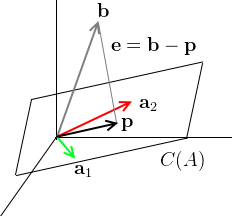
- $\mathbf b$ is not on the plane $C(A)$, but we project on it to get $\mathbf p$
- $\mathbf e = \mathbf b - \mathbf p$ is our projection error
$\mathbf e$ - want to make it as small as possible,
- so $\mathbf e \; \bot \; \text{plane}$ or $\mathbf b - \mathbf p \; \bot \; \text{plane}$
- we want to find what combinations of the basis vectors $\mathbf a_1$ and $\mathbf a_2$ will make $\mathbf p$
- thus we express $\mathbf p$ as $\mathbf p = \hat x_1 \mathbf a_1 + \hat x_2 \mathbf a_2$
- since these $\mathbf a_1$ and $\mathbf a_2$ are from the matrix $A$, we can write $\mathbf p = A \mathbf{\hat x}$
- so the goal is to find the right combinations of $\mathbf a_1$ and $\mathbf a_2$ s.t. $\mathbf e \; \bot \; \text{plane}$
Now we’re solving $\mathbf p = A \mathbf{\hat x}$
- how to find $\mathbf{\hat x}$?
- $\mathbf e = \mathbf b - \mathbf p = \mathbf b - A \mathbf{\hat x}$,
- $\mathbf e \; \bot \; \text{plane}$, or $\mathbf e \; \bot \; \mathbf a_1$ and $\mathbf e \; \bot \; \mathbf a_2$ - $\mathbf e$ is orthogonal to every vector in $C(A)$
- if vectors are orthogonal, their Dot Product is zero. So now we have two equations:
- $\mathbf a_1^T (\mathbf b - A \mathbf{\hat x}) = 0$
- $\mathbf a_2^T (\mathbf b - A \mathbf{\hat x}) = 0$
- let’s write it in the matrix form:
- $A^T = \begin{bmatrix}
- \ \mathbf a_1^T - \
- \ \mathbf a_2^T -
\end{bmatrix}$- $\begin{bmatrix}
- \ \mathbf a_1^T - \
- \ \mathbf a_2^T -
\end{bmatrix} \cdot (\mathbf b - A \mathbf{\hat x}) = \begin{bmatrix} 0
0
\end{bmatrix}$- or $A^T \mathbf e = \mathbf 0$
-
thus $\mathbf e \in N(A^T)$ - the projection error belongs to the left nullspace - and we know that $C(A) \; \bot \; N(A^T)$ (see Space Orthogonality) - 
Let’s solve it
- $A^T \mathbf e = \mathbf 0$, $\mathbf e = \mathbf b - \mathbf p = \mathbf b - A \mathbf{ \hat x}$
- so $A^T (\mathbf b - A \mathbf{\hat x}) = 0$
- $A^T \mathbf b - A^T A \mathbf{\hat x} = 0$
- $A^T A \mathbf{\hat x} = A^T \mathbf b$
- or $\mathbf{\hat x} = (A^T A)^{-1} A^T \mathbf b$
- $A^T A$ is invertible when $A$ has independent columns (see the theorem below)
The projection $\mathbf p$
- this way we found the coefficients $\mathbf{\hat x}$, but not the projection $\mathbf p$
- we need to take all vectors of $C(A)$ (columns of $A$) and scale by $\mathbf{\hat x}$
- thus we have $\mathbf p = A \mathbf{\hat x} = A (A^T A)^{-1} A^T \mathbf b$
-
recall the 1-dim case: $\mathbf p = x \cdot \mathbf a = \mathbf a \cdot \cfrac{\mathbf a^T \mathbf b}{\mathbf a^T \mathbf a}$ - it’s very similar
-
Projection Matrix
How do we use a nice matrix representation for projecting onto subspaces?
- we introduce a ‘‘Projection’’ matrix $P$ that projects from one subspace to another
Projecting on a Line
It’s $\mathbb R^n \to \mathbb R^1$ case
Let $P$ be the projection matrix, i.e.
- $P$ s.t. $\mathbf p = P \mathbf b$ - a matrix $P$ with which we can express the Linear Transformation that brings $\mathbf b$ to $\mathbf p$
- we know that $\mathbf p = \mathbf a \cdot \cfrac{\mathbf a^T \mathbf b}{\mathbf a^T \mathbf a}$
- so $\mathbf p = P \mathbf b$ or $P = \cfrac{\mathbf a \mathbf a^T}{\mathbf a^T \mathbf a}$
-
in the numerator we have an Outer Product, and we have an Inner Product in the denominator - it’s $| \mathbf a |^2$
Properties
- it’s normalized rank-1 matrix
- $\text{dim } C(P) = 1$, it consists of a line through $\mathbf a$, and $\mathbf a$ is the basis for $C(P)$
- $P$ is symmetric:
- $P^T = \left( \cfrac{\mathbf a \mathbf a^T}{\mathbf a^T \mathbf a} \right)^T = \cfrac{1}{\mathbf a^T \mathbf a} (\mathbf a \mathbf a^T)^T = \cfrac{1}{\mathbf a^T \mathbf a} \mathbf a^T (\mathbf a^T)^T = \cfrac{\mathbf a \mathbf a^T}{\mathbf a^T \mathbf a} = P$
- what happens if we project something twice?
- it shouldn’t do anything the 2nd time
- so $\mathbf p = P \cdot \mathbf b = P \cdot P \cdot \mathbf b$
- or $P^2 = P$
General Case
It’s $\mathbb R^n \to \mathbb R^k$ case
- from the previous example we learned that $\mathbf p = A \mathbf{\hat x} = A (A^T A)^{-1} A^T \mathbf b$
- so it means that $P = A (A^T A)^{-1} A^T$
Note:
- we cannot expand $(A^T A)^{-1}$ as $A^{-1} (A^T)^{-1}$ because we assume that $A$ is not invertible
- if $A$ is invertible, then it would span the entire space and $P = I$
Properties
$P$ from $n$-dim has the same properties as $P$ for 1-dim
- $P^T = P$
- $P^2 = P$
- $P^2 = \Big(A (A^T A)^{-1} A^T \Big) \cdot \Big(A (A^T A)^{-1} A^T \Big) = A (A^T A)^{-1} \cancel{A^T A (A^T A)^{-1}} A^T = A (A^T A)^{-1} A^T = P$
We want to project $\mathbf b$.
- if $\mathbf b \in C(A)$ then $P \mathbf b = \mathbf b$
- $\mathbf b \in C(A)$ $\Rightarrow$ $\mathbf b$ is a combination of columns of $A$
- so $\mathbf b = A \mathbf x$, thus $p = P \mathbf b = A (A^T A)^{-1} A^T \mathbf p = A \cancel{(A^T A)^{-1} A^T A} \mathbf x = A \mathbf x = \mathbf b$
- if $\mathbf b \; \bot \; C(A)$ then $P \mathbf b = \mathbf 0$
- $\mathbf b \; \bot \; C(A) \Rightarrow A^T \mathbf b = \mathbf 0$ or $\mathbf b \in N(A^T)$
- $P \mathbf b = A (A^T A)^{-1} \underbrace{A^T \mathbf b}_{\mathbf 0} = \mathbf 0$
$P$ as an action of $A$
We can show the projection matrix $P$ as an action performed on $A$
- in terms of pictures, here’s what $P$ does:

Picture
- $\mathbf b \not \in C(A)$ so cannot solve $A \mathbf x = \mathbf b$.
- project on $C(A)$: solve $A^T A \mathbf{\hat x} = A^T \mathbf b$ instead
- at the same time, there’s another part of $\mathbf b$ - it’s $\mathbf e \in N(A^T)$, $\mathbf b = \mathbf p + \mathbf e$
- $\mathbf b = P \mathbf b + \mathbf e$
- $\mathbf e$ is also a projection of $\mathbf b$, but on $N(A^T)$
- the projection matrix is $(I - P) \mathbf b$ - this is the projection onto space orthogonal to $A$
- check: $\mathbf p + \mathbf e = P \mathbf b + (I - P) \mathbf b = \mathbf b$
- $(I - P)$ is a projection matrix, so it obeys all the rules and properties of projection matrices
When $P$ projects on some subspace, $I - P$ projects onto the perpendicular subspace
Theorem: $A^T A$ is Invertible
See this theorem in Gram Matrices
Projection onto Orthogonal Basis
Let $\mathbf q_1, \ … \ , \mathbf q_n \in \mathbb R^m$ be a set of orthonormal vectors
-
$Q = \Bigg[ \mathop{\mathbf q_1}\limits_ ^ \ \mathop{\mathbf q_2}\limits_ ^ \ \cdots \ \mathop{\mathbf q_n}\limits_ ^ \Bigg]$. It’s an Orthogonal Matrix - suppose we want to project on the subspace $C(Q)$ - Projection matrix $P$, usual case: $P = A (A^T A)^{-1} A^T$
- For orthogonal matrices $Q^T Q = I$, so $P = Q (Q^T Q)^{-1} Q^T = Q Q^T$
Thus, to project $\mathbf b$ onto $C(Q)$ we do this: $\mathbf p = P \mathbf b$
- $\mathbf p = P \mathbf b = Q (Q^T \mathbf b) = \Bigg[ \mathop{\mathbf q_1}\limits_| ^| \ \mathop{\mathbf q_2}\limits_|^| \cdots \ \mathop{\mathbf q_n}\limits_|^| \Bigg] \begin{bmatrix} |\mathbf q_1^T \mathbf b
\vdots
\mathbf q_n^T \mathbf b
\end{bmatrix} = \mathbf q_1 (\mathbf q_1^T \mathbf b) + \ … \ + \mathbf q_n (\mathbf q_n^T \mathbf b)$
What if $m = n$?
- $Q$ is square and then $Q Q^T = I$ as well
- That means that $P = I$, i.e. the basis spans the entire space
- but still, $\mathbf b = \mathbf q_1 (\mathbf q_1^T \mathbf b) + \ … \ + \mathbf q_n (\mathbf q_n^T \mathbf b)$
- why is it useful? because it enables us to decompose a vectors into perpendicular pieces
- this is the foundation of the Fourier Transformation| | |
Applications
- Normal Equation in Linear Least Squares
- Fourier Transformation
Sources
- Linear Algebra MIT 18.06 (OCW)
- The Four Fundamental Subspaces: 4 Lines, G. Strang, [http://web.mit.edu/18.06/www/Essays/newpaper_ver3.pdf]
- The fundamental theorem of linear algebra, G. Strang [http://www.engineering.iastate.edu/~julied/classes/CE570/Notes/strangpaper.pdf]
- Strang, G. Introduction to linear algebra.
- http://physics-help.info/physicsguide/appendices/vectors.shtml
- http://en.wikipedia.org/wiki/Linear_least_squares_%28mathematics%29