Precision and Recall

Precision and Recall

Precision and Recall are quality metrics used across many domains:

originally it’s from Information Retrieval
also used in Machine Learning

Precision and Recall for Information Retrieval

IR system has to be:

precise: all returned document should be relevant
efficient: all relevant document should be returned

Given a test collection, the quality of an IR system is evaluated with:

'’Precision’’: % of relevant documents in the result
'’Recall’’: % of retrieved relevant documents

More formally,

given a collection of documents $C$
If $X \subseteq C$ is the output of the IR system and $Y \subseteq C$ is the list of all relevant documents then define
'’precision’’ as $P = \cfrac- both $P$ and $R$ are defined w.r.t a set of retrieved documents

Precision/Recall Curves

If we retrieve more document, we improve recall (if return all docs, $R = 1$)
if we retrieve fewer documents, we improve precision, but reduce recall
so there’s a trade-off between them

Let $k$ be the number of retrieved documents

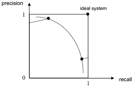
then by varying $k$ from $0$ to $N =

$ we can draw $P$ vs $R$ and obtain the Precision/recall curve:

source: [http://www.searchtechnologies.com/precision-recall]

the closer the curve to the $(1, 1)$ point - the better the IR system performance
source: Information Retrieval (UFRT) lecture 2

Area under P/R Curve:

Analogously to ROC Curves we can calculate the area under the P/R Curve
the closer AUPR to 1 the better

Average Precision

Top-$k$-precision is insensitive to change of ranks of relevant documents among top $k$

how to measure overall performance of an IR system?

$\text{avg P} = \cfrac{1}{K} \sum_{k = 1}^K \cfrac{k}{r_k}$

where $r_i$ is the rank of $k$th relevant document in the result

Since in a test collection we usually have a set of queries, we calcuate the average over them and get Mean Average Precision: MAP

Precision and Recall for Classification

The precision and recall metrics can also be applied to Machine Learning: to binary classifiers

+ Diagnostic Testing Measures [http://en.wikipedia.org/wiki/Template:DiagnosticTesting_Diagram]

colspan=”2” rowspan=”2” style=”border:none;”

colspan=”2”

Actual Class $y$

Positive

Negative

rowspan=”2”

$h_{\theta}(x)$
Test
outcome

Test
outcome
positive

style=”background:#ccffcc;”

’'’True positive’’‘
($\text{TP}$)

style=”background:#eedddd;”

’'’False positive’’‘
($\text{FP}$, Type I error)

Precision =
$\cfrac{# \text{TP}}{# \text{TP} + # \text{FP}}$

Test
outcome
negative

style=”background:#eedddd;”

’'’False negative’’‘
($\text{FN}$, Type II error)

style=”background:#ccffcc;”

’'’True negative’’‘
($\text{TN}$)

Negative predictive value =
$\cfrac{# \text{TN}}{# \text{FN} + # \text{TN}}$

colspan=”2” style=”border:none;”

Sensitivity =
$\cfrac{# \text{TP}}{# \text{TP} + # \text{FN}}$

Specificity =
$\cfrac{# \text{TN}}{# \text{FP} + # \text{TN}}$

Accuracy =
$\cfrac{# \text{TP} + # \text{TN}}{# \text{TOTAL}}$

Main values of this matrix:

’'’True Positive’’’ - we predicted “+” and the true class is “+”
’'’True Negative’’’ - we predicted “-“ and the true class is “-“
’'’False Positive’’’ - we predicted “+” and the true class is “-“ (Type I error)
’'’False Negative’’’ - we predicted “-“ and the true class is “+” (Type II error)

Two Classes: $C_+$ and $C_-$

Precision

$\pi = P\big(f(\mathbf x) = C_+ \, \big \, h_{\theta}(\mathbf x) = C_+ \big)$ - given that we predict $\mathbf x$ is +
what’s the probability that the decision is correct
we estimate precision as $P = \cfrac{\text{# TP}}{\text{# predicted positives}} = \cfrac{\text{# TP}}{\text{# TP} + \text{# FP}}$

Interpretation

Out of all the people we thought have cancer, how many actually had it?
High precision is good
we don’t tell many people that they have cancer when they actually don’t

Recall

$\rho = P\big(h_{\theta}(\mathbf x) = C_+ \, \big \, f(\mathbf x) = C_+ \big)$ - given a positive instance $\mathbf x$
what’s the probability that we predict correctly
we estimate recall as $R = \cfrac{\text{# TP}}{\text{# actual positives}} = \cfrac{\text{# TP}}{\text{# TP + # FN}}$

Interpretation

Out of all the people that do actually have cancer, how much we identified?
The higher the better:
We don’t fail to spot many people that actually have cancer
For a classifier that always returns zero (i.e. $h_{\theta}(x) = 0$) the Recall would be zero
That gives us more useful evaluation metric
And we’re much more sure

F Measure

$P$ and $R$ don’t make sense in the isolation from each other

higher level of $\rho$ may be obtained by lowering $\pi$ and vice versa

Suppose we have a ranking classifier that produces some score for $\mathbf x$

we decide whether to classify it as $C_+$ or $C_-$ based on some threshold parameter $\tau$
by varying $\tau$ we will get different precision and recall
improving recall will lead to worse precision
improving precision will lead to worse recall
how to pick the threshold?
combine $P$ and $R$ into one measure (also see ROC Analysis)

$F_\beta = \cfrac{(\beta^2 + 1) P\, R}{\beta^2 \, P + R}$

$\beta$ is the tradeoff between $P$ and $R$
if $\beta$ is close to 0, then we give more importance to $P$
- $F_0 = P$
if $\beta$ is closer to $+ \infty$, we give more importance to $R$

When $\beta = 1$ we have $F_1$ score:

The $F_1$-score is a single measure of performance of the test.
it’s the harmonic mean of precision $P$ and recall $R$
$F_1 = 2 \cfrac{P \, R}{P + R}$

Motivation: Precision and Recall

Let’s say we trained a Logistic Regression classifier

we predict 1 if $h_{\theta}(x) \geqslant 0.5$
we predict 0 if $h_{\theta}(x) < 0.5$

Suppose we want to predict y = 1 (i.e. people have cancer) only if we’re very confident

we may change the threshold to 0.7
- we predict 1 if $h_{\theta}(x) \geqslant 0.7$
- we predict 0 if $h_{\theta}(x) < 0.7$
We’ll have higher precision in this case (all for who we predicted y = 1 are more likely to actually have it)
But lower recall (we’ll miss more patients that actually have cancer, but we failed to spot them)

Let’s consider the opposite

Suppose we want to avoid missing too many cases of y=1 (i.e. we want to avoid false negatives)
So we may change the threshold to 0.3
- we predict 1 if $h_{\theta}(x) \geqslant 0.3$
- we predict 0 if $h_{\theta}(x) < 0.3$
That leads to
Higher recall (we’ll correctly flag higher fraction of patients with cancer)
Lower precision (and higher fraction will turn out to actually have no cancer)

Questions

Is there a way to automatically choose the threshold for us?
How to compare precision and recall numbers and decide which algorithm is better?
at the beginning we had a single number (error ratio) - but now have two and need to choose which one to prefer
$F_1$ score helps to decide since it’s just one number

Example

Suppose we have 3 algorithms $A_1$, $A_2$, $A_3$, and we captured the following metrics:

$P$ !! $R$ !! $\text{Avg}$ !! $F_1$

$A_1$

0.5

0.4

0.45

0.444

$\leftarrow$ our choice

$A_2$

0.7

0.1

0.4

0.175

$A_3$

0.02

1.0

0.54

0.0392

Here’s the best is $A_1$ because it has the highest $F_1$-score

Precision and Recall for Clustering

Can use precision and recall to evaluate the result of clustering

Correct decisions:

’'’TP’’’ = decision to assign two similar documents to the same cluster
’'’TN’’’ = assign two dissimilar documents to different clusters

Errors:

’'’FP’’’: assign two dissimilar documents to the same cluster
’'’FN’’’: assign two similar documents to different clusters

So the confusion matrix is:

same !! different

same

different

Example

Consider the following example (from the IR book [http://nlp.stanford.edu/IR-book/html/htmledition/evaluation-of-clustering-1.html])

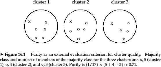
there are $\cfrac{n \, (n - 1)}{2} = 136$ pairs of documents
$\text{TP} + \text{FP} = {6 \choose 2} + {6 \choose 2} + {5 \choose 2} = 40$
$\text{TP} = {5 \choose 2} + {4 \choose 2} + {3 \choose 2} + {2 \choose 2} = 20$
etc

So have the following contingency table:

same !! different

same

$\text{TP} = 20$

$\text{FN} = 24$

different

$\text{FP} = 20$

$\text{TN} = 72$

Thus,

$P = 20/40 = 0.5$ and $R = 20/44 \approx 0.455$
$F_1$ score is $F_1 \approx 0.48$

Multi-Class Problems

How do we adapt precision and recall to multi-class problems?

let $f(\cdot)$ be the target unknown function and $h_\theta(\cdot)$ the model
let $C_1, \ … , C_K$ be labels we want to predict ($K$ labels)

Precision w.r.t class $C_i$ is

$P\big(f(\mathbf x) = C_i \ \big \ h_\theta(\mathbf x) = C_i \big)$ - probability that given that we classified $\mathbf x$ as $C_i$
the decision is indeed correct

Recall w.r.t. class $C_i$ is

$P\big(h_\theta(\mathbf x) = C_i \ \big \ f(\mathbf x) = C_i \big)$ - given an instance $\mathbf x$ belongs to $C_i$
what’s the probability that we predict correctly

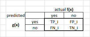
We estimate these probabilities using a contingency table w.r.t each class $C_i$

Idea similar to the One-vs-All Classification technique

Contingency Table for $C_i$:

let $C_+$ be $C_i$ and
let $C_-$ be all other classes except for $C_i$, i.e. $C_- = { C_j } - C_i$ (all classes except for $i$)
then we create a contingency table
and calculate $\text{TP}_i, \text{FP}_i, \text{FN}_i, \text{TN}_i$ for them

Now estimate precision and recall for class $C_i$

$P_i = \cfrac{\text{TP}_i}{\text{TP}_i + \text{FP}_i}$
$R_i = \cfrac{\text{TP}_i}{\text{TP}_i + \text{FN}_i}$

Averaging

These precision and recall are calculated for each class separately
how to combine them?

’'’Micro-averaging’’’

calculate TP, … etc globally and then average
let
- $\text{TP} = \sum_i \text{TP}_i$
- $\text{FP} = \sum_i \text{FP}_i$
- $\text{FN} = \sum_i \text{FN}_i$
- $\text{TN} = \sum_i \text{TN}_i$
and then calculate precision and recall as
- $P^\mu = \cfrac{\text{TP}}{\text{TP} + \text{FP}}$
- $R^\mu = \cfrac{\text{TP}}{\text{TP} + \text{FN}}$

’'’Macro-averaging’’’

calculate $P_i$ and $R_i$ “locally” for each $C_i$
and then let $P^M = \cfrac{1}{K} \sum_i P_i$ and $R^M = \cfrac{1}{K} \sum_i R_i$

Micro and macro averaging behave quite differently and may give different results

the ability to behave well on categories with low generality (fewer training examples) will be less emphasized by macroaveraging
which one to use? depends on application

This way is often used in Document Classification

Sources

Machine Learning (coursera)
Sebastiani, Fabrizio. “Machine learning in automated text categorization.” (2002). [http://arxiv.org/pdf/cs/0110053.pdf]
Zhai, ChengXiang. “Statistical language models for information retrieval.” 2008.
Information Retrieval (UFRT)
Manning, Christopher D., Prabhakar Raghavan, and Hinrich Schütze. “Introduction to information retrieval.” 2008. [http://informationretrieval.org/]

✏️ Edit on GitHub