ROC Analysis

ROC Analysis

ROC stands for ‘'’R’'’eceiver ‘'’O’'’perating ‘'’C’'’haracteristic (from Signal Detection Theory)

initially - for distinguishing noise from not noise
so it’s a way of showing the performance of Binary Classifiers
- only two classes - noise vs not noise
it’s created by plotting the fraction of True Positives vs the fraction of False Positives
- True Positive Rate, $\text{tpr} = \cfrac{\text{TP}}{\text{TP} + \text{FN}}$ (sometimes called “sensitivity” or “recall”)
- False Positive Rate $\text{fpr} = \cfrac{\text{FP}}{\text{FP} + \text{TN}}$ (also Fall-Out)
- see Evaluation of Binary Classifiers

Evaluation of Binary Classifiers

precision and recall are popular metrics to evaluate the quality of a classification system
ROC Curves can be used to evaluate the tradeoff between true- and false-positive rates of classification algorithms

Properties:

ROC Curves are insensitive to class distribution
If the proportion of positive to negative instances changes, the ROC Curve will not change

ROC Space

When evaluating a binary classifier, we often use a Confusion Matrix

however here we need only TPR and FPR
$\text{tpr} = \cfrac{\text{TP}}{\text{TP} + \text{FN}}$
- Fraction of positive examples correctly classified
$\text{fpr} = \cfrac{\text{FP}}{\text{FP} + \text{TN}}$
- Fraction of negative examples incorrectly classified
ROC space is 2DIM:
- $X: \text{fpr}, Y: \text{tpr}$

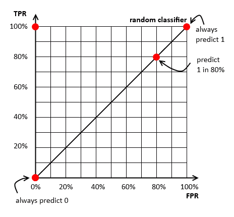
ROC Space Baseline

Baseline

for the baseline we put a random classifier that predicts 1 with some probability
e.g. on the illustration we have 3 random classifiers:
always predict 0 (0% change to predict 1)
predict 1 in 80% cases
always predict 1 (in 100% cases)

In practice, we can never obtain a classifier below this line

suppose we have a classifier $C_1$ below the line with $\text{fpr} = 80\%$, and $\text{tpr} = 30\%$
can make it better than random by inverting its prediction:
$C_2(x)$: if $C_1(x) = 1$, return 0; if $C_1(x) = 0$, return 1
position on the ROC Space of $C_2$ is $(1 - \text{fpr}, 1 - \text{tpr}) = (20\%, 70\%)$
roc-inv.png

Multi-Class Classifier

If you have a multi-class classifier, use One-vs-All Classification

e.g. for 3 classes $C_1, C_2, C_3$ build 3 ROC spaces

ROC Space

Positive

$C_1$

$C_2$

$C_3$

Negative

$C_2 \cup C_3$

$C_1 \cup C_3$

$C_1 \cup C_2$

ROC Convex Hull

Suppose we have 5 classifiers $C_1, C_2, …, C_5$

we calculate $\text{fpr}$ and $\text{tpr}$ for each and plot them on one plot

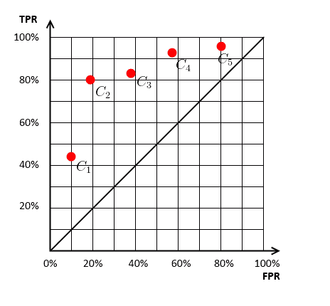
Then we can try to find classifiers that achieve the best $\text{fpr}$ and $\text{tpr}$

by the Dominance principle, we have the following Pereto frontier
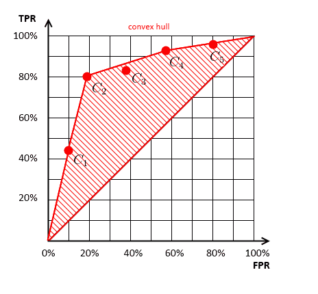
this is called the “ROC Convex Hull”
classifiers below this Hull are always suboptimal
e.g. $C_3$ is always worse than anything else

ISO Accuracy Lines

There’s a simple relationship between accuracy and $\text{fpr}$, $\text{tpr}$: notation:

$N$ the # of examples,
$\text{NEG}$ - # of negative examples, and $\text{POS}$ - # of positive examples
$\text{neg}$ - fraction of negative examples, $\text{pos}$ - fraction of positive examples

$\text{acc} = \text{trp} \cdot \text{pos} + \text{neg} - \text{neg} \cdot \text{fpr}$

$\text{acc} = \cfrac{\text{TP} + \text{TN}}{N} = \cfrac{\text{TP}}{N} + \cfrac{\text{TN}}{N} = \cfrac{\text{TP}}{\text{POS}} \cdot \cfrac{\text{POS}}{N} + \cfrac{\text{NEG} - \text{FP}}{N} = \cfrac{\text{TP}}{\text{POS}} \cdot \cfrac{\text{POS}}{N} + \cfrac{\text{NEG}}{N} - \cfrac{\text{FP}}{\text{NEG}} \cdot \cfrac{\text{NEG}}{N} = \text{trp} \cdot \text{pos} + \text{neg} - \text{neg} \cdot \text{fpr}$
so can rewrite this and get
- $\text{tpr} = \cfrac{\text{acc} - \text{neg}}{\text{pos}} + \cfrac{\text{neg}}{\text{pos}} \cdot \text{fpr}$
it’s a line: $y = ax + b$
- $y = \text{tpr}, x = \text{fpr}, a = \cfrac{\text{neg}}{\text{pos}}, x = \cfrac{\text{neg}}{\text{pos}}, b = \cfrac{\text{acc} - \text{neg}}{\text{pos}}$

Property

the ratio $\text{neg} / \text{pos}$ is the slope $a$ of our line
- changing this ratio we can have many slopes
and changing accuracy we can obtain many parallel lines with the same slope
higher lines are better

to calculate the corresponding accuracy

find the intersection point of the accuracy line (red)
and the descending diagonal (blue)

+ Examples

$\text{neg} / \text{pos}$

Accuracy Lines

$\text{neg} / \text{pos} = 1$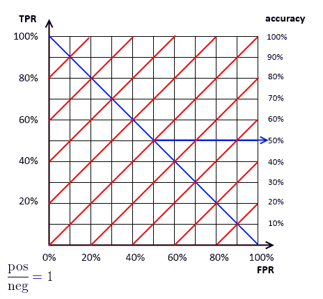

$\text{neg} / \text{pos} = 0.5$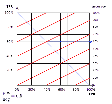

ISO Accuracy Lines vs Convex Hull

Recall this picture:

this the convex hull of the ROC plot

Each line segment of the ROC Convex Hull is an ISO accuracy line

for a particular class distribution (slope) and accuracy
- all classifiers on a line achieve the same accuracy for this distribution
$\text{neg} / \text{pos} > 1$
- distribution with more negative examples
- the slope is steep
- classifier on the left is better
$\text{neg} / \text{pos} < 1$
- distribution with more positive examples
- the slope is flatter
- classifier on the right is better

Each classifier on the convex hull is optimal

w.r.t. accuracy
for a specific distribution

Selecting the Optimal Classifier

First, we need to know the ratio $\text{neg} / \text{pos}$

given it, we can find the classifier that achieves the highest accuracy for this ratio
fix the ratio, keep increasing accuracy until reach the end of the hull

Distribution

Best Classifier

Accuracy

ISO Accuracy Line

$\text{neg} / \text{pos} = 1/1$

$C_2$

$\approx$ 81%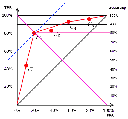

$\text{neg} / \text{pos} = 1/4$

$C_4$

$\approx$ 83%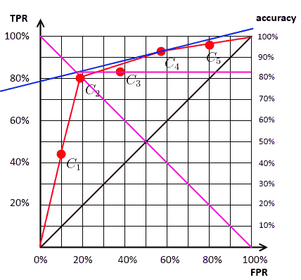

$\text{neg} / \text{pos} = 4/1$

$C_4$

$\approx$ 81%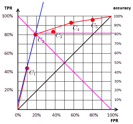

ROC Curves

Scoring Classifiers

A scoring classifier (or ranker) is an algorithm that

instead of one single label it outputs the scores for each class
and you take the label with the highest score
e.g.: Naive Bayes Classifier, Neural Networks, etc

For binary classification

ranker $F$ outputs just a single number
have to set some threshold $\theta$ to transform the raker into a classifier
- positive class if $F(X, +) > \theta$
e.g. like in Logistic Regression
how to set a threshold?
- use Cross-Validation for fining the best value for $\theta$
- or draw ROC Curves, producing a point in the ROC Space for each possible threshold

ROC Curve

plot of $\text{fpr}$ vs $\text{tpr}$ for different thresholds of the same ranker
a model with perfect discrimination passes through the upper left corner
- '’perfect discrimination’’ - with no overlap between the two classes
so the closer the ROC curve to the upper corner, the better the accuracy

Naive Method

Algorithm

given a ranker $F$ and a dataset $S$ with $N$ training examples
consider all possible thresholds ($N-1$ for $N$ examples)
for each,
- calculate $\text{fpr}$ and $\text{tpr}$
- and put in on the ROC space
select the best, using the ROC Analysis
- knowing the ratio $\text{neg} / \text{pos}$

Practical Method

Algorithm

rank test examples on decreasing score $F(x, +) $
start in $(0, 0)$
for each example $x$ (in the decreasing order)
- if $x$ is positive, move $1/\text{pos}$ up
- if $x$ is negative, move $1/\text{neg}$ right

Example 1

Given

20 examples: https://www.dropbox.com/s/65rdiv42ixe2eac/roc-lift.xlsx
$C$ - actual class of the training example
$\text{pos} / \text{neg} = 1$, i.e. $1/\text{pos} = 1/\text{neg} = 0.1$

Best threshold

we know the slope of the accuracy line: it’s 1
the best classifier for this slope is the 6th one
threshold value $\theta$
- so we take the score obtained on the 6th record
- and use it as the threshold value $\theta$
- i.e. predict positive if $\theta \geqslant 0.54$
if we check, we see that indeed we have accuracy = 0.7

Example 2

Given

20 training examples, 12 negative and 8 positive

| # | Cls | Score | 1 | N | 0.18 || 2 | N | 0.24 || 3 | N | 0.32 || 4 | N | 0.33 || 5 | N | 0.4 || 6 | N | 0.53 || 7 | N | 0.58 || 8 | N | 0.59 || 9 | N | 0.6 || 10 | N | 0.7 || 11 | N | 0.75 || 12 | N | 0.85 || 13 | P | 0.52 || 14 | P | 0.72 || 15 | P | 0.73 || 16 | P | 0.79 || 17 | P | 0.82 || 18 | P | 0.88 || 19 | P | 0.9 || 20 | P | 0.92 |

$\Rightarrow$ sort by score

| # | Cls | Score | 20 | P | 0.92 || 19 | P | 0.9 || 18 | P | 0.88 || 12 | N | 0.85 || 17 | P | 0.82 || 16 | P | 0.79 || 11 | N | 0.75 || 15 | P | 0.73 || 14 | P | 0.72 || 10 | N | 0.7 || 9 | N | 0.6 || 8 | N | 0.59 || 7 | N | 0.58 || 6 | N | 0.53 || 13 | P | 0.52 || 5 | N | 0.4 || 4 | N | 0.33 || 3 | N | 0.32 || 2 | N | 0.24 || 1 | N | 0.18 |

Now draw the curves: -

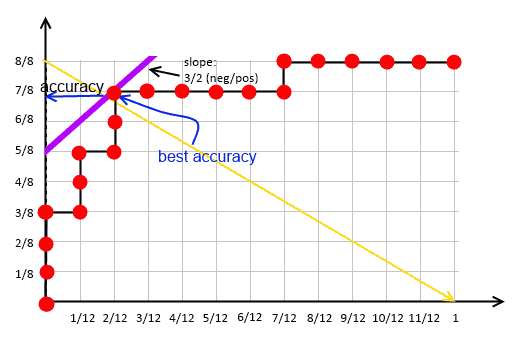- best accuracy achieved with example # 18 - so setting $\theta$ to 0.88 - obtained accuracy is $15/20$

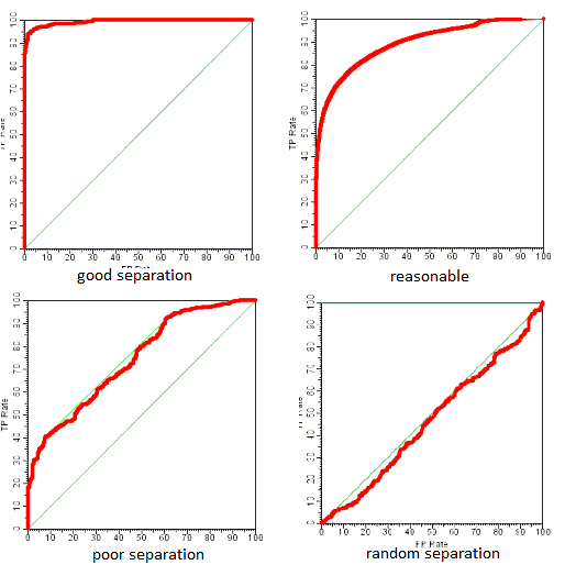
Other ROC Curve Examples

Taken from [http://www.cs.bris.ac.uk/~flach/ICML04tutorial/ROCtutorialPartI.pdf]

AUC: Area Under ROC Curve

Area Under ROC Curve

Measure for evaluating the performance of a classifier
it’s the area under the ROC Curve

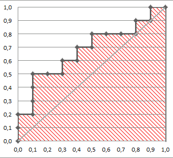
total area is 100%

so AUC = 1 is for a perfect classifier for which all positive come after all negatives
AUC = 0.5 - randomly ordered
AUC = 0 - all negative come before all positive
so AUC $\in [0, 1]$
typically we don’t have classifiers with AUC < 0.5

Interpretation

Formally, the AUC of a classifier $C$ is

probability that $C$ ranks a randomly drawn “$+$” example higher than a randomly drawn “$-$” example
i.e. $\text{auc}(C) = P \big[ C(x^+) > C(x^-) \big]$

Consider the ROC curve above (auc=0.68).

Let’s make an experiment
draw random positive and negative examples
then calculate the proportion of cases when positives have greater score than negatives
at the end, we obtain 0.67926 - quite close to 0.68| | | ```bash cls = c(‘P’, ‘P’, ‘N’, ‘P’, ‘P’, ‘P’, ‘N’, ‘N’, ‘P’, ‘N’, ‘P’, ‘N’, ‘P’, ‘N’, ‘N’, ‘N’, ‘P’, ‘N’, ‘P’, ‘N’) score = c(0.9, 0.8, 0.7, 0.6, 0.55, 0.51, 0.49, 0.43, 0.42, 0.39, 0.33, 0.31, 0.23, 0.22, 0.19, 0.15, 0.12, 0.11, 0.04, 0.01)

pos = score[cls == ‘P’] neg = score[cls == ‘N’]

set.seed(14) p = replicate(50000, sample(pos, size=1) > sample(neg, size=1)) mean(p)

 


### Examples
Examples:
- have a look at the examples in [#Other ROC Curve Examples](#Other_ROC_Curve_Examples)
- we see that the better classifier is, the bigger the area under its ROC curve
- and for the random one it's apparent that it's 0.5

## ROC Analysis in [R](R)
### ROC Curves
In R there's a package called ROCR [http://cran.r-project.org/web/packages/ROCR/index.html] for drawing ROC Curves

```bash
install.packages('ROCR')
require('ROCR')

cls = c('P', 'P', 'N', 'P', 'P', 'P', 'N', 'N', 'P', 'N', 'P', 
        'N', 'P', 'N', 'N', 'N', 'P', 'N', 'P', 'N')
score = c(0.9, 0.8, 0.7, 0.6, 0.55, 0.51, 0.49, 0.43, 
          0.42, 0.39, 0.33, 0.31, 0.23, 0.22, 0.19, 
          0.15, 0.12, 0.11, 0.04, 0.01)


pred = prediction(score, cls)
roc = performance(pred, "tpr", "fpr")

plot(roc, lwd=2, colorize=TRUE)
lines(x=c(0, 1), y=c(0, 1), col="black", lwd=1)

AUC

With ROCR it’s as well possible to calculate AUC:

auc = performance(pred, "auc")
auc = unlist(auc@y.values)
auc

Cutoff Plots

Also, can generate a plot of accuracy vs threshold - to select the best threshold. Suppose we have the following ROC curve:

For that we can plot accuracy vs cutoff plot:

So the best cutoff is at around 0.5 for this graph

path = 'https://raw.githubusercontent.com/alexeygrigorev/datasets/master/wiki-r/roc/columns.txt'
cols = read.table(path, sep='\t', header=T, dec='.', as.is=T)

cols$score = as.numeric(cols$score)


library(ROCR)

pos = table(cols$class)['1']
neg.sample = sample(which(cols$class == 0), pos)

cols.sample = data.frame(score=c(cols$score[cols$class == 1], 
                                 cols$score[neg.sample]),
                         class=c(rep(1, pos), rep(0, pos)))

pred = prediction(cols.sample$score, cols.sample$class)
roc = performance(pred, "tpr", "fpr")

plot(roc, colorize=T, lwd=2)
lines(x=c(0, 1), y=c(0, 1), col="grey", lty=2)


auc = performance(pred, "auc")
auc = unlist(auc@y.values)
auc

acc = performance(pred, "acc")

ac.val = max(unlist(acc@y.values))
th = unlist(acc@x.values)[unlist(acc@y.values) == ac.val]

plot(acc)
abline(v=th, col='grey', lty=2)

ROC in Java

AUC Calculation

(This code uses LambdaJ [https://code.google.com/p/lambdaj/] for grouping and soring)

```component pascal private static final int NEGATIVE = 0; private static final int POSITIVE = 1;

public static double auc(List list) { List data = sort(list, on(TrainingInstance.class).getPredictedScore(), DESCENDING);

Group group = group(data, by(on(TrainingInstance.class).getCls())); double tpr = 1.0 / group.find(POSITIVE).size(); double fpr = 1.0 / group.find(NEGATIVE).size();

double auc = 0.0; double height = 0.0;

for (TrainingInstance ti : data) { if (ti.getCls() == POSITIVE) { height = height + tpr; } else { auc = auc + height * fpr; } }

return auc; } ```

Sources

Data Mining (UFRT)
http://www.cs.bris.ac.uk/~flach/ICML04tutorial/ROCtutorialPartI.pdf
http://www.medcalc.org/manual/roc-curves.php

✏️ Edit on GitHub

ROC Analysis

ROC Analysis

ROC Space

ROC Space Baseline

Multi-Class Classifier

ROC Convex Hull

ISO Accuracy Lines

ISO Accuracy Lines vs Convex Hull

Selecting the Optimal Classifier

ROC Curves

Scoring Classifiers

Naive Method

Practical Method

Example 1

Example 2

Other ROC Curve Examples

AUC: Area Under ROC Curve

Interpretation

AUC

Cutoff Plots

ROC in Java

AUC Calculation

See Also

Links

Sources