Simulation in R
Distributions
| Name | Function | Density | | rbeta | dbeta || Binomial Distribution | rbinom | dbinom || | rcauchy | dcauchy || | rchisq | dchisq || | rexp | dexp || | rf | df || | rgamma | dgamma || | rgeom | dgeom || | rhyper | dhyper || | rlogis | dlogis || | rlnorm | dlnorm || | rnbinom | dnbinom || Normal Distribution | rnorm | dnorm || | rpois | dpois || | rt | dt || Uniform Distribution | runif | dunif || | rweibull | dweibull |
rname: Distribution Function
Generates 10 random values from Normal Distribution
- with standard deviation 3 and mean 188
```text only heights = rnorm(10, mean=188, sd=3)
186.0 191.2 187.6 187.9 186.6 187.2 187.2 189.5 190.8 186.4 ```
Generates 10 random values from Binomial Distribution
- flipping a coin 10 times:
- of 10 independent experiments with probability 0.5
```text only coinFlips = rbinom(10,size=10,prob=0.5)
3 4 6 5 7 6 5 8 5 6 ```
dname: Probability Density Function
Calculates the density of some probability distribution ```text only x = seq(from=-5, to=5, length=10) normalDensity = dnorm(x, mean=0, sd=1) round(normalDensity, 2) [1] 0.00 0.00 0.01 0.10 0.34 0.34 0.10 0.01 0.00 0.00
same with 15 :
```text only
x = seq(from=-3, to=3, length=15)
normalDensity = dnorm(x, mean=0, sd=1)
r = round(normalDensity, 2)
bp = barplot(r)
xspline(x=bp, y=r, lwd=2, shape=1, border="blue")
text(x=bp, y=r+0.03, labels=as.character(r), xpd=TRUE, cex=0.7)
Code [https://stat.ethz.ch/pipermail/r-help/2003-November/041967.html
So we can see that it generates the values of the density function
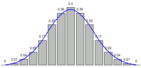
- may be useful for Statistical Tests of Significance
Same for the Binomial distribution:
```text only x = seq(0,10,by=1) binomialDensity = dbinom(x,size=10,prob=0.5) round(binomialDensity,2)
## [Sampling](Sampling)
Function <code>sample</code> draws a random sample
- <code>function(x, size, replace= FALSE, prob = NULL) </code>
- <code>replace = T</code> for sampling with replacement

```text only
s = seq(0, 20)
> 0  1  2  3  4  5  6  7  8  9 10 11 12 13 14 15 16 17 18 19 20
sample(s, size=10)
> 8  4 11 12 20  7 19 18  1 14
sample(s, size=10, replace=T)
> 6 17 18  7  2  9 18  0  7  5
Note that 7 and 18 are selected twice for the sample with replacement
The sample can be draw with specified probability
- e.g. suppose we want to sample with normal distribution
```text only dnorm(seq(-3, 3, length=length(s))) sample(s, size=10, replace=T, prob=n)
9 7 11 11 1 13 11 14 5 6 ```
- note that 11 gets selected 3 times,
- because the probability of selecting it is quite high: 0.3989
Reproducibility
When we experiment, we typically want to reproduce it later
- so it’s important to generate the same “random” data
- for that we can set the seed for PRG
set.seed(12345)