Gram-Schmidt Process

$\require{cancel}$

Gram-Schmidt Process

In Linear Algebra, Gram-Schmidt process is a method for orthogonalization:

• given a matrix $A$ it produces an Orthogonal Matrix $Q$ from it
• $A$ must have linearly independent columns

2D Case

Suppose we have two linearly independent vectors $\mathbf a$ and $\mathbf b$

• we want to make them orthogonal $\mathbf a \Rightarrow \mathbf v_1$, $\mathbf b \Rightarrow \mathbf v_2$
• and then we normalize them: $\mathbf v_1 \Rightarrow \mathbf q_1$ and $\mathbf v_2 \Rightarrow \mathbf q_2$
• 
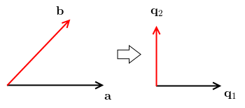
• $\mathbf a$ is already fine, let’s keep its direction for $\mathbf q_1$ as well
• $\mathbf b$ is not fine: we want it to be orthogonal to $\mathbf q_1$

How do we produce a vector $\mathbf v_2$ from $\mathbf b$ such that $\mathbf v_2 \; \bot \; \mathbf v_1 = \mathbf a$

• 
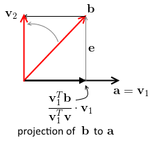
• let’s project $\mathbf b$ on $\mathbf v_1$, and we get $P \cdot \mathbf v_1 = \cfrac{\mathbf v_1^T \mathbf b}{\mathbf v_1^T \mathbf v_1} \cdot \mathbf v_1$
• $\mathbf e$ is our projection error, so $\mathbf e = \mathbf b - P \mathbf v_1 = \mathbf b - P \mathbf v_1 = \mathbf b - \cfrac{\mathbf v_1^T \mathbf b}{\mathbf v_1^T \mathbf v_1} \cdot \mathbf v_1$

• note that $\mathbf v_2 = \mathbf e$

  it has the same length and the same direction

  - so $\mathbf v_2 = \mathbf b - \cfrac{\mathbf v_1^T \mathbf b}{\mathbf v_1^T \mathbf v_1} \cdot \mathbf v_1$

  - interpretation: we take the original vector $\mathbf b$ and remove the projection of this vector onto $\mathbf v_1$, and it leaves only the orthogonal part

• now $\mathbf v_1 \; \bot \mathbf v_2$
• let’s check: $\mathbf v_1^T \mathbf v_2 = \mathbf v_1^T \left( \mathbf b - \cfrac{\mathbf v_1^T \mathbf b}{\mathbf v_1^T \mathbf v_1} \cdot \mathbf v_1 \right) = \mathbf v_1^T \mathbf b - \mathbf v_1^T \cdot \cfrac{\mathbf v_1^T \mathbf b}{\mathbf v_1^T \mathbf v_1} \cdot \mathbf v_1 = \mathbf v_1^T \mathbf b - \mathbf v_1^T \mathbf b = 0$

To find the final solution, we just normalize $\mathbf v_1$ and $\mathbf v_2$:

• $\mathbf q_1 = \mathbf v_1 / | \mathbf v_1 |$

  - $\mathbf q_2 = \mathbf v_2 / | \mathbf v_2 |$

3D Case

What if we have 3 vectors $\mathbf a, \mathbf b, \mathbf c$?

• need to find (pair-wise) orthogonal vectors $\mathbf v_1, \mathbf v_2, \mathbf v_3$ and then normalize them
• have $\mathbf v_1 = a$, $\mathbf v_2 = \mathbf b - \cfrac{\mathbf v_1^T \mathbf b}{\mathbf v_1^T \mathbf v_1} \mathbf v_1$
• what about $\mathbf v_3$? Know that we want to have $\mathbf v_3 \; \bot \; \mathbf v_1$ and $\mathbf v_3 \; \bot \; \mathbf v_2$
• for $\mathbf v_3$, we want to subtract its components in direction $\mathbf v_1$ as well as in direction $\mathbf v_2$
• so $\mathbf v_3 = \mathbf c - \cfrac{\mathbf v_1^T \mathbf c}{\mathbf v_1^T \mathbf v_1} \cdot \mathbf v_1 - \cfrac{\mathbf v_2^T \mathbf c}{\mathbf v_2^T \mathbf v_2} \cdot \mathbf v_2$

To get $\mathbf q_1, \mathbf q_2, \mathbf q_3$, we just normalize:

• $\mathbf q_1 = \mathbf v_1 / | \mathbf v_1 |$

  - $\mathbf q_2 = \mathbf v_2 / | \mathbf v_2 |$

  - $\mathbf q_3 = \mathbf v_3 / | \mathbf v_3 |$

3D Case Animation

File:Gram-Schmidt_orthonormalization_process.gif

Source:

Column Spaces

Claim: The column space of $A$ does not change when we orthogonalize it

QR Factorization

We can think of the Gram-Schmidt Process in the matrix language (like for Gaussian Elimination that brings us to LU Factorization)

• recall that $C(Q) = C(A)$
• because of this, there exists a third matrix $R$ that brings $A$ to $Q$
• or, $A = Q R$
• (so we want Gram-Schmidt applied to the columns of $A$)

How to find this $R$?

• $A = QR$, let’s multiply both sides by $Q^T$:
• $Q^T A = Q^T Q R$
• since $Q^T Q = I$, we have $R = Q^T A$
• let $A = \Bigg[ \mathop{\mathbf a_1}\limits_| ^| \ \mathop{\mathbf a_2}\limits_|^| \ \cdots \ \mathop{\mathbf a_n}\limits_|^| \Bigg]$ and $Q = \Bigg[ \mathop{\mathbf q_1}\limits_|^| \ \mathop{\mathbf q_2}\limits_|^| \ \cdots \ \mathop{\mathbf q_n}\limits_|^| \Bigg]$ |- thus we have $R = Q^T A = \begin{bmatrix} \mathbf q_1^T \mathbf a_1 & \mathbf q_1^T \mathbf a_2 & \cdots & \mathbf q_1^T \mathbf a_n
  \mathbf q_2^T \mathbf a_1 & \mathbf q_2^T \mathbf a_2 & \cdots & \mathbf q_2^T \mathbf a_n
  \vdots & \vdots & \ddots & \vdots
  \mathbf q_n^T \mathbf a_1 & \mathbf q_n^T \mathbf a_2 & \cdots & \mathbf q_n^T \mathbf a_n
  \end{bmatrix}$

Now recall the way we constructed $Q$

• we took $\mathbf q_1 = \mathbf a_1 / | \mathbf a_1 |$ and make all other $\mathbf a_i$ orthogonal to it, so $\mathbf q_2^T \mathbf a_1 = \ … \ = \mathbf q_n^T \mathbf a_1 = 0$

  - then we took $\mathbf q_1$ and $\mathbf q_2$ and made all $\mathbf a_3, …, \mathbf a_n$ orthogonal to them, so $\mathbf q_3^T \mathbf a_2 = \ … \ = \mathbf q_n^T \mathbf a_2 = 0$

• proceeding this way till the end we see that $R$ is upper-diagonal:
• thus we have $R = Q^T A = \begin{bmatrix} \mathbf q_1^T \mathbf a_1 & \mathbf q_1^T \mathbf a_2 & \cdots & \mathbf q_1^T \mathbf a_n
  0 & \mathbf q_2^T \mathbf a_2 & \cdots & \mathbf q_2^T \mathbf a_n
  \vdots & \vdots & \ddots & \vdots
  0 & 0 & \cdots & \mathbf q_n^T \mathbf a_n
  \end{bmatrix}$

Note that for the diagonal elements of $R$, $\mathbf q_i^T \mathbf a_i = | \mathbf v_i |$ |- why?

• 

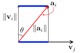
• $\mathbf q_i^T \mathbf a_i = | \mathbf q_i | | \mathbf a_i | \cos \theta$ by the Dot Product definition

  - $| \mathbf q_i | = 1$ and $\cos \theta = \cfrac{| \mathbf v_i - $\mathbf q_i^T \mathbf a_i = | \mathbf q_i | | \mathbf a_i | \cos \theta = 1 \cdot \cancel{| \mathbf a_i - this can be uses to speed up the computation a bit

Usage

This is often used for Linear Least Squares - to make the Normal Equation faster

Implementation code

Python

Implementation of the pseudo-code from the Strang’s book:

import numpy as np

def qr_factorization(A):
  m, n = A.shape
  Q = np.zeros((m, n))
  R = np.zeros((n, n))

  for j in range(n):
    v = A[:, j]
        
    for i in range(j - 1):
      q = Q[:, i]
      R[i, j] = q.dot(v)
      v = v - R[i, j] * q

    norm = np.linalg.norm(v)
    Q[:, j] = v / norm
    R[j, j] = norm
  return Q, R

A = np.random.rand(13, 10) * 1000
Q, R = qr_factorization(A)

Q.shape, R.shape
np.abs((A - Q.dot(R)).sum()) < 1e-6

Sources

• Linear Algebra MIT 18.06 (OCW)
• Strang, G. Introduction to linear algebra.
• http://en.wikipedia.org/wiki/Gram%E2%80%93Schmidt_process
• http://inst.eecs.berkeley.edu/~ee127a/book/login/l_mats_qr.html