Singular Value Decomposition

linear-algebra matrix-decomposition

Singular Value Decomposition

SVD is a decomposition of rectangular $m \times n$ matrix $A$ as

$A = U \Sigma V^T$ where
$U$ is an $m \times m$ orthogonal matrix with Eigenvectors of $A A^T$
$\Sigma$ is an diagonal $m \times n$ matrix with Eigenvalues of both $A^T A$ and $A A^T$
$V$ is an $n \times n$ orthogonal matrix with Eigenvalues of $A^T A$

Orthogonal Basis for the Four Fundamental Subspaces

But it’s not only a decomposition, but a way of finding the bases for the Four Fundamental Subspaces of $A$:

Singular vectors $\mathbf v_1, \ … \ , \mathbf v_r$ are in the row space of $A$
applying $A$ to $\mathbf v_i$ gives $A \mathbf v_i = \sigma_i \mathbf u_i$
$\mathbf u_1, \ … \ , \mathbf u_r$ are in the column space of $A$
Singular values $\sigma_1, \ … \ , \sigma_r$ are all positive numbers
so $V$ and $U$ diagonalize $A$:
$A \mathbf v_i = \sigma_i \mathbf u_i$ $\Rightarrow$ $A V = \Sigma U$
The singular values $\sigma_i$ in $\Sigma$ are arranged in monotonic non-increasing order

EVD vs SVD

Eigenvalue Decomposition

Problems with general Eigendecomposition $A = S \, \Lambda \, S^{-1}$:

doesn’t work with rectangular matrices
eigenvalues in $S$ are usually not orthonormal (unless $A$ is symmetric)

Our goal:

$A = U \Sigma V^T$
we want to find the orthogonal basis in the Row Space $C(A^T)$ of $A$
and we then map this basis to some orthogonal basis in the Column Space $C(A)$ of $A$
these vectors are called ‘‘singular vectors’’

Solution:

choose basis from $AA^T$ and $A^T A$ - they are symmetric and have orthonormal basis

Spectral Theorem

SVD extends the Spectral Theorem

it’s EVD for all symmetric positive-definite matrices
we extend EVD to all rectangular matrices $A$

Finding SVD

Goal:

find orthonormal bases in the row space of $A$ as well as in the column space of $A$
s.t. $A$ maps from row space basis to the column space basis
and the matrix $A$ is diagonal w.r.t. this basis

Orthogonalization

Finding orthogonal basis for the rowspace $C(A^T)$

let $r$ be the rank of $A$
select orthonormal basis $\mathbf v_1, \ … \ , \mathbf v_r$ in $\mathbb R^n$ s.t. it spans the Row Space of $A$
e.g. using the Gram-Schmidt Process on the rows of $A^T$
continue the process to find $\mathbf v_{r+1}, \ … \ , \mathbf v_n$ in $\mathbb R^n$ s.t it spans the Nullspace of $A$

Then for $i = 1 .. r$ define $\mathbf u_i$ as $A \mathbf v_i$

i.e. $A \mathbf v_i = \sigma_i \mathbf u_i$
extend this to a basis in $\mathbb R^m$
relative to these bases, $A$ will have diagonal representation

Here ${ \ \mathbf v_i \ }$ are orthogonal by construction

but ${ \ \mathbf u_i \ }$ aren’t necessarily orthogonal
we want to find such ${ \ \mathbf v_i \ }$ that ${ \ \mathbf u_i \ }$ are also orthogonal

We can use EVD to find the right basis

Let ${ \ \mathbf v_i \ }$ be eigenvectors of $A^T A$ with $\lambda_i$ being corresponding eigenvalues
so $A^T A \mathbf v_i = \lambda_i \mathbf v_i$ and EVD is $A^T A = V \Lambda V^T$ (with $\mathbf v_i$ being the columns of $V$)

Will it give the right bases?

the Inner Product $\langle A \mathbf v_i, A \mathbf v_j \rangle$ is $(A \mathbf v_i)^T (A \mathbf v_j) = \mathbf v_i^T A^T A \mathbf v_j = \mathbf v_i^T (A^T A \mathbf v_j) = \mathbf v_i^T \lambda_j \mathbf v_j = \lambda_j \mathbf v_i^T \mathbf v_j$
if $i \ne j$, then $\mathbf v_i^T \mathbf v_j =0$
so the image $\big{ A \mathbf v_1, \ … \ , A \mathbf v_n \big}$ is also orthogonal

Finding the orthonormal ${ \ \mathbf u_i \ }$

vectors $A \mathbf v_i$ are orthogonal, but not orthonormal

$| A \mathbf v_i |^2 = \langle A \mathbf v_i, A \mathbf v_i \rangle = \mathbf v_i^T A^T A \mathbf v_i = \mathbf v_i^T \lambda_i \mathbf v_i = \lambda_i$

- let $\mathbf u_i = \cfrac{A \mathbf v_i}{| A \mathbf v_i - if $r < m$, we extend this basis for $\mathbb R^m$

This completes the construction for the bases

Let $\sigma_i = \sqrt{\lambda_i}$. Then $\mathbf u_i = \cfrac{1}{\sigma_i} A \mathbf v_i$
or $A \mathbf v_i = \sigma_i \mathbf u_i$
Put ${ \mathbf v_1, \ … \ , \mathbf v_r }$ in columns of $V$ and ${ \mathbf u_1, \ … \ , \mathbf u_r }$ in columns of $U$
so we’ll have $A V = U \Sigma$
thus, SVD is $A = U \Sigma V^T$

Summary:

$A$ is $m \times n$ real matrix
express $A = U \Sigma V^T$
$V$ is obtained from diagonal factorization $A^T A = V \Lambda V^T$
$U$ is normalized image $\big{ A \mathbf v_1, \ … \ , A \mathbf v_n \big}$
non-zero entries $\sigma_i$ of $\Sigma$ are square roots of $\lambda_i$ from $\Lambda$: $\sigma_i = \sqrt{\lambda_i}$

This construction shows that SVD exists, but it doesn’t mean that it’s the most effective way of implementing it

the computation of $A^T A$ can lead to loss of precision (because of the way numbers are stored in memory)
there are direct methods of computing SVD on $A$, without having to compute $A^T A$

There’s duality: we can do the save for $AA^T$:

EVD is $AA^T = U \Lambda U^T$, $\mathbf u_i$ are columns of $U$
let’s apply $A^T$ to these $\mathbf u_i$
The image of this tranformation is also orthogonal: $\langle A^T \mathbf u_i, A^T \mathbf u_j \rangle = \lambda_i$ if $i = j$ and $0$ otherwise
we normalize $A^T \mathbf u_i$ by $\sigma_i = \sqrt{\lambda_i}$
so it’s completely the same, but coming from the column space side

$\Sigma$: Eigenvalues of $A^T A$ and $AA^T$

What is more, the eigenvalues of $A^T A$ and $AA^T$ are the same| | |Let’s first show that if $\lambda$ is eigenvalue for $A^T A$, then it’s an eigenvalue for $AA^T$

let $\lambda \ne 0$ be an eigenvalue of $A^T A$ with corresponding eigenvector $\mathbf v \ne \mathbf 0$
then $A^T A \mathbf v = \lambda \mathbf v$. Multiply by $A$ on the left:
$A A^T A \mathbf v = \lambda A \mathbf v$
let $\mathbf u = A \mathbf v$, then $A A^T \mathbf u = \lambda \mathbf u$
so $\lambda$ is an eigenvalue for $A A^T$ as well, with eigenvector $\mathbf u = A \mathbf v$

Now show that if $\lambda$ is eigenvalue for $AA^T$ then it’s also eigenvalue for $A^T A$

same idea as before
let $\lambda \ne 0$ be an eigenvalue of $A A^T$ with corresponding eigenvector $\mathbf u \ne \mathbf 0$
then $A A^T \mathbf u = \lambda \mathbf u$. Multiply by $A^T$ on the left
$A^T A A^T \mathbf u = \lambda A^T \mathbf u$
by letting $\mathbf v = A^T \mathbf u$ we have $A^T A \mathbf v = \lambda \mathbf v$
so $\lambda$ is an eigenvalue for $A A^T$ as well, with eigenvector $\mathbf v = A^T \mathbf u$

$\square$

Calculating eigenvalues

So, for example, if $A$ is $500 \times 2$, then $AA^T$ is $500 \times 500$ and $A^T A$ is $2 \times 2$
we calculate eigenvalues for $A^T A$, (there are 2 of them)
and we know that $AA^T$ has the same 2 eigenvalues - with the rest 498 being 0

Reconstructing EVD from SVD

We saw how to construct SVD using EVD, but we can also reconstruct EVD from SVD

let $A = U \Sigma V^T$, then
$A^T A = V \Sigma^T \Sigma V^T = V \Sigma^2 V^T$ is EVD of $A^T A$
$A A^T = U \Sigma \Sigma^T U^T = U \Sigma^2 U^T$ is EVD of $A A^T$
where $\Sigma^T \Sigma = \Sigma \Sigma^T = \Sigma^2 = \text{diag}(\sigma_1^2, \ … \ , \sigma_r^2)$

If $A$ is square and symmetric, then $A = A^T$ and $A^T A = A A^T = A^2$

and any eigenvector $\mathbf v$ of $A$ with eigenvalue $\lambda$ is eigenvector of $A^2$ with eigenvalue $\lambda^2$
so $U = V$ and EVD = SVD when $A$ is positive semi-definite (no negative eigenvalues)

Geometric Interpretation

Let’s understand how $A$ deforms the space

consider a unit sphere in $\mathbb R^n$
a vector $\mathbf x \in \mathbb R^n$ is represented as $\mathbf x = \sum x_i \mathbf v_i$
because it’s a sphere, $\sum x_i^2 = 1$
then the image $A \mathbf x = \sum x_i A \mathbf v_i = \sum x_i A \mathbf v_i = \sum \sigma_i x_i \mathbf u_i$
let $y_i = x_i \sigma_i$
then $A \mathbf x = \sum y_i \mathbf u_i$
$\sum\limits_{i = 1}^r \cfrac{y_i^2}{\sigma_i^2} = \sum\limits_{i = 1}^r x_i^2 \leqslant 1$
if $A$ has full rank, then the sum is strictly $1$

So $A$ maps the unit sphere in $\mathbb R^n$ to some $r$-dimensional ellipsoid in $\mathbb R^m$ with axes in directions $\mathbf u_i$, each with magnitudes $\sigma_i$

Linear transformation:
So first it collapses $n - r$ dimensions of the domain
then it distorts the remaining dimensions stretching and squeezing the $r$-dim unit sphere into an ellipsoid
finally it embeds the ellipsoid into $\mathbb R^m$
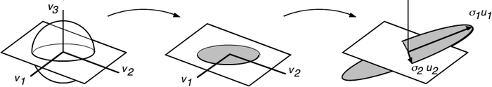
From (Kalman96)
$n = m = 3$, $r = 2$

Another way:

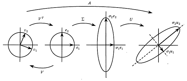
From (Strang93)

Representation

Partitioned Matrices

Let’s have a look at $A = U \Sigma V^T$ for $m \times n$ matrix $A$:

$A = \left[ \begin{array}{cccc| ccc} || & | & & | & | & & | \ || & | & & | & | & & | \ |\mathbf u_1 & \mathbf u_2 & \cdots & \mathbf u_r & \mathbf u_{r+1} & \cdots & \mathbf u_m \ | & | & & | & | & & | \ || & | & & | & | & & | \ |\end{array} \right] \left[ \begin{array}{cccc| ccc} |\sigma_1 & & & &
& \sigma_2 & & & &
& & \ddots & & &
& & & \sigma_r & &
\hline & & & & 0 &
& & & & & \ddots &
& & & & & & 0
\end{array} \right] \begin{bmatrix}
& \mathbf v_1^T & -
& \vdots & \
& \mathbf v_1^T & -
\hline
& \mathbf v_{r+1}^T & -
& \vdots & \
& \mathbf v_n^T & -
\end{bmatrix}$
Then using Matrix Multiplication for block-partitioned matrices, we see that
$A = \begin{bmatrix} | & | & & | \ |\mathbf u_1 & \mathbf u_2 & \cdots & \mathbf u_r \ | & | & & | \ |\end{bmatrix} \begin{bmatrix} \sigma_1 & &
& \sigma_2 & &
& & \ddots &
& & & \sigma_r
\end{bmatrix} \begin{bmatrix}
& \mathbf v_1^T & -
& \vdots & \
& \mathbf v_1^T & -
\end{bmatrix} + \begin{bmatrix} | & & | \ |\mathbf u_{r+1} & \cdots & \mathbf u_m \ | & & | \ |\end{bmatrix} \begin{bmatrix} 0 & &
& \ddots &
& & 0
\end{bmatrix} \begin{bmatrix}
& \mathbf v_{r+1}^T & -
& \vdots & \
& \mathbf v_n^T & -
\end{bmatrix}$
so, $A = \begin{bmatrix} | & | & & | \ |\mathbf u_1 & \mathbf u_2 & \cdots & \mathbf u_r \ | & | & & | \ |\end{bmatrix} \begin{bmatrix} \sigma_1 & &
& \sigma_2 & &
& & \ddots &
& & & \sigma_r
\end{bmatrix} \begin{bmatrix}
& \mathbf v_1^T & -
& \vdots & \
& \mathbf v_1^T & -
\end{bmatrix} $
so only first $r$ $\mathbf v_i$’s and $\mathbf u_i$’s contribute something
now $U$ and $V$ become rectangular and $\Sigma$ square:

SVD is $A = U \Sigma V^T$

$U$ is $m \times r$ matrix s.t. $U^T U = I$
$\Sigma$ is $r \times r$ diagonal matrix $\text{diag}(\sigma_1, \ … \ , \sigma_r)$
$V$ is $n \times r$ matrix s.t. $V^T V = I$

Outer Product Form

A matrix multiplication $AB$ can be expressed as a sum of outer products:

let $A$ be $n \times k$ matrix and $B$ be $k \times m$ matrix
then $AB = \sum\limits_{i=1}^k \mathbf a_i \mathbf b_i^T$
where $\mathbf a_i$ are columns of $A$ and $\mathbf b_i$ are rows of $B$

Thus we can represent $A = U \Sigma V^T$ as sum of outer products:

$A = \sum\limits_{i = 1}^r \sigma_i \mathbf u_i \mathbf v_i^T$

It gives another way of thinking about the Linear Tranformation $f(\mathbf x) = A \mathbf x$

$A \mathbf x = (\sum \sigma_i \mathbf u_i \mathbf v_i^T) \mathbf x = \sum \sigma_i \mathbf u_i (\mathbf v_i^T \mathbf x) = \sum \sigma_i (\mathbf v_i^T \mathbf x) \mathbf u_i$
so we express $A \mathbf x$ as a linear combination of ${ \ \mathbf u_i \ }$

Truncated SVD

Usual SVD:

$A = U \Sigma V$
$\sigma_i$ in $\text{diag}(\Sigma)$ are in non-increasing order
so we can keep only first $k$ singular values of $\Sigma$ (and set the rest to 0) and get the best rank-$k$ approximation of $A$
this is the best approximation in terms of Total Least Squares (see Reduced Rank Approximation)

In terms of sum of rank-1 matrices, we can approximate $A$ by

$A_k = \sum_{i = 1}^k \sigma_i \mathbf u_i \mathbf v_i^T$

Properties & Questions

Column Space and Row Space

Given SVD $A V = U \Sigma$, why $U$ in is the column space of $A$ and $V$ is the row space?

For all $i$: $A \mathbf v_i = \sigma_i \mathbf u_i$. Since there’s a solution, then $\sigma_i \mathbf u_i \in C(A)$
for all $i$: $A^T \mathbf u_i = \sigma_i \mathbf v_i$. Then $\sigma_i \mathbf u_i \in C(A^T)$ which is the row space of $A$

Applications

Dimensionality Reduction

Principal Component Analysis

PCA is often implemented through SVD

Data Compression

Truncated SVD gives the best rank-$k$ approximation to the original matrix $A$
when using Frobenius Norm in the Matrix Vector Space
the problem is Reduced Rank Approximation (sometimes Total Least Squares)

It’s like Discrete Fourier Transformation:

in DFT we represent a data vector in orthogonal basis of sines and cosines
often there are only a few principal frequencies that account for most variability in the data and the rest can be discarded
SVD does the same, but it find the best orthogonal basis instead of using a predefined one
so we can see SVD as adaptive generalization of DFT

Image Compression

images can be represented as Matrices, so we can apply SVD and PCA to them
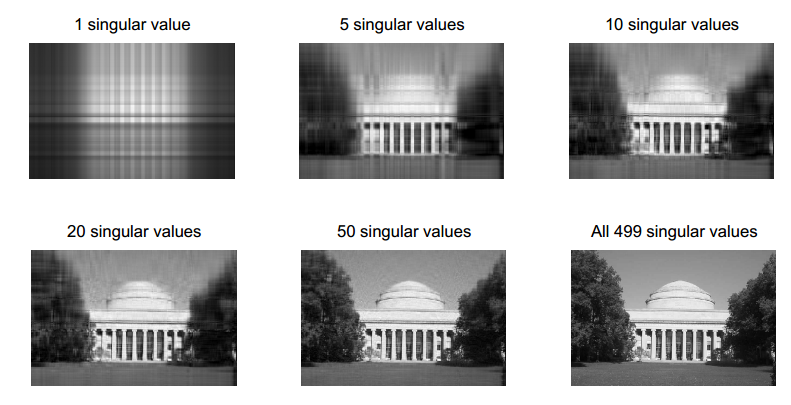
source: SVD at work [from http://web.mit.edu/18.06/www/extras.shtml

Latent Semantic Analysis

When used as a Dimensionality Reduction technique for Term-Document matrix
it helps revealing some hidden semantic patterns

Linear Least Squares

As a technique for faster Normal Equation computation

but generally QR Decomposition is better, but sometimes less stable

Others

There are many other applications

Sources

Linear Algebra MIT 18.06 (OCW)
Strang, G. Introduction to linear algebra.
Jauregui, Jeff. “Principal component analysis with linear algebra.” (2012). [http://www.math.union.edu/~jaureguj/PCA.pdf]
Kalman, Dan. “A singularly valuable decomposition: the SVD of a matrix.” (1996). [http://www.math.washington.edu/~morrow/498_13/svd.pdf]
Strang, Gilbert. “The fundamental theorem of linear algebra.” (1993). [http://www.engineering.iastate.edu/~julied/classes/CE570/Notes/strangpaper.pdf]

✏️ Edit on GitHub

Singular Value Decomposition