Support Vector Machines
SVM vs Logistic Regression
Recall Logistic Regression:
- the hypothesis is of the form $h_{\theta}(x) = g(\theta^T x) = \cfrac{1}{1 + e^{-\theta^T x}}$
- if $y = 1$ we want $h_{\theta}(x) \approx 1$, or $\theta^T x \gg 0$
- if $y = 0$ we want $h_{\theta}(x) \approx 0$, or $\theta^T x \ll 0$
Cost Function
Logistic Regression cost function is
- $\text{cost}(h_{\theta}(x), y) = \left{\begin{array}{l l} -\log(h_{\theta}(x)) & \text{ if } y = 1 \ - \log(1 - h_{\theta}(x)) & \text{ if } y = 0 \end{array} \right. $
- let’s have a look at contribution of each part of the cost function:
- $- \log \cfrac{1}{1 + e^{-z}}$: if $y = 1$, it gives $\theta^T x \gg 0$
- $- \log \left(1 - \cfrac{1}{1 + e^{-z}} \right)$: if $y = 0$, it gives $\theta^T x \ll 0$
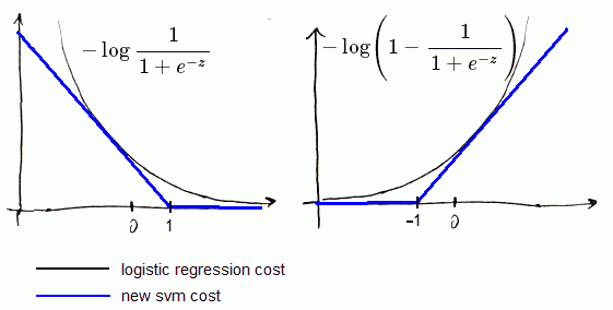
Let’s change that function onto 2 straight lines:
- one with some slope,
- and second is flat (see the picture)
That gives us
- an approximation of the regression function
- computational advantages and
- easier optimization
Objective Function
for Logistic Regression we had
- $J(\theta) = \cfrac{1}{m} \sum_{i = 1}^{m} \left [ y^{(i)} \cdot \text{cost}{1}(\theta^T x^{(i)}) + (1 - y^{(i)}) \cdot \text{cost}{0}(\theta^T x^{(i)}) \right] + \cfrac{\lambda}{2m} \sum_{j = 1}^{n} \theta_j^2$
- where $\text{cost}{1}(\theta^T x^{(i)})$ and $\text{cost}{0}(\theta^T x^{(i)})$ are logarithmic cost functions for $y = 1$ and $y = 0$ respectively.
- Let’s change them onto svm’s cost functions $\text{cost}{1}(\theta^T x^{(i)})$ and $\text{cost}{0}(\theta^T x^{(i)})$
- Now, to transform it to svm’s objective function:
- we multiply it by $m$,
- divide by $\lambda$,
- and let $C = \cfrac{1}{\lambda}$
Finally we have:
- $J(\theta) = C \cdot \sum_{i = 1}^{m} \left [ y^{(i)} \cdot \text{cost}{1}(\theta^T x^{(i)}) + (1 - y^{(i)}) \cdot \text{cost}{0}(\theta^T x^{(i)}) \right] + \cfrac{1}{2} \sum_{j = 1}^{n} \theta_j^2$
- This is just different convention and it doesn’t change the value of $\theta$ that minimizes this function
Hypothesis
The final difference is that
- Logistic Regression outputs probabilities
-
- but for SVM out hypothesis is
- $h_{\theta}(x) = \left{ \begin{array}{l l} 1 & \text{ if } \theta^T x \geqslant 0 \ 0 & \text{ otherwise } \end{array} \right.$
Large Margin
- Here’s the SVM cost functions:
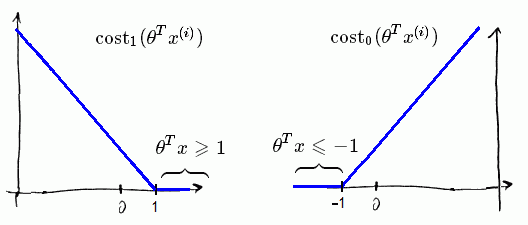
Large margin means that
- when $y = 1$ we want $\theta^T x \geqslant 1$, not just $\geqslant 0$
- when $y = 0$ we want $\theta^T x \leqslant -1$, not just $< 0$
That gives larger margin for SVM
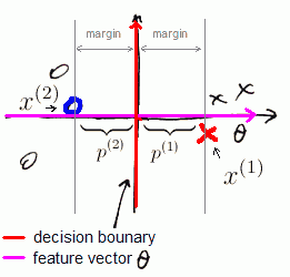
SVM Decision Boundary
- SVM sometimes is referred as Large Margin classifier
- The reason for that is SVM tries to find a decision boundary that has the widest distance (‘‘margin’’ from the dataset samples)
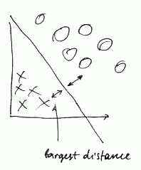
- here we see the margin
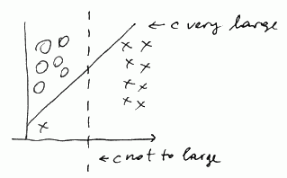
When $C$ is big, the algorithm becomes sensitive to outliers, decreasing $C$ makes it less sensitive
Math Behind It
For SVM, suppose our cost function is
- $J(\theta) = \cfrac{1}{2} \sum_{j = 1}^{n} \theta_j^2$ s.t.
- $\theta^T x^{(i)} \geqslant 1$ if $y^{(i)} = 1$ and
- $\theta^T x^{(i)} \leqslant -1$ if $y^{(i)} = 0$
- For simplification we skip the fist term of our sum and we assume that $\theta_0 = 0$ and number of features $n = 2$
- $\theta^2 = \theta^T \theta$ is an Inner Product
-
- so we get:
- $J(\theta) = \cfrac{1}{2} \sum_{j = 1}^{n} \theta_j^2 = \cfrac{1}{2} (\theta_1^2 + \theta_2^2) = \cfrac{1}{2} \left( \sqrt{\theta_1^2 + \theta_2^2} \right)^2 = \cfrac{1}{2} | \theta |^2$ |- our optimization objective is to minimize the norm of $\theta$| | | Next, let’s have a look at $\theta^T \cdot x^{(i)}$
- this is Inner Product as well
- let $p^{(i)}$ be projection from $x^{(i)}$ to $\theta$
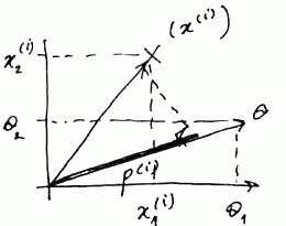
- $\theta^T \cdot x^{(i)} = \theta_1 x_1^{(i)} + \theta_2 x_2^{(i)} $
- It means that we can replace the constraints $\theta^T x^{(i)} \geqslant 1$ on $p^{(i)} | \theta | \geqslant 1$ | Thus we get the following optimization objective:
- $\min_{\theta} \cfrac{1}{2} \sum_{j = 1}^{n} \theta_j^2$, s.t.
-
$p^{(i)} \cdot | \theta | \geqslant 1$ if $y^{(i)} = 1$ - $p^{(i)} \cdot | \theta | \leqslant -1$ if $y^{(i)} = 0$
-
Suppose we have the following decision boundary
But SVM will never give us such line
- both $p^{(1)}$ and $p^{(2)}$ are small numbers (see the picture)
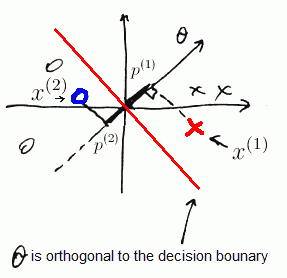
- $\Rightarrow$ $| \theta |$ has to be large| | | Let’s now imagine that SVM chooses
- $OY$ axis as a decision boundary and
- vector $\theta$ is orthogonal - goes along $OX$
Here again we have
- $p^{(1)} > 0$ and $p^{(2)} < 0$, but they are much bigger now
- $| \theta |$ doesn’t have to be big | That is how SVM gets large margins: because our projections are large.
As a simplification, we assumed $\theta_0 = 0$
- which just means that the boundary always goes through the origin (0, 0)
- if $\theta_0 \neq 0$, it will simply mean that the boundary doesn’t pass (0, 0) but otherwise works in exactly same way
Kernels
'’Kernels’’ is a technique for using a SVN as a complex, non-linear classifier
Suppose we have the following data
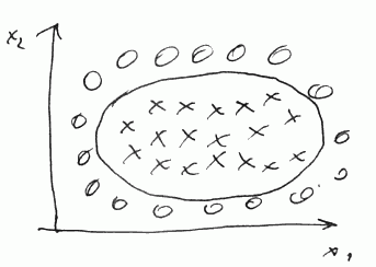
- The decision boundary is non linear
-
- so we predict $y = 1$ if
- $\theta_0 + \theta_1 x_1 + \theta_2 x_2 + \theta_3 x_1 x_2 + \theta_4 x_1^2 + + \theta_5 x_2^2 + … \geqslant 0$
Let’s denote each feature as $f$:
- $f_1 = x_1$, $f_2 = x_2 $, $f_3 = x_1 x_2$, $f_4 = x_1^2$, $f_5 = x_2^2$
-
- So we have
- $\theta_0 + \theta_1 f_1 + \theta_2 f_2 + \theta_3 f_1 f_2 + \theta_4 f_1^2 + \theta_5 f_2^2 + … \geqslant 0$
Is there a different / better choice of features $f_1, f_2, f_3, …$?
Similarity
Say our $x \in \mathbb{R}^2$
- We may pick up 3 data points, or ‘‘landmarks’’: $l^{(1)}, l^{(2)}, l^{(3)}$
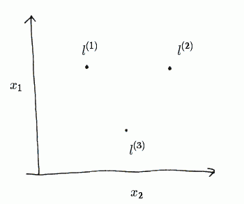
- So given a new $x$ we compute new features as proximity to these $l^{(1)}$, $l^{(2)}$ and $l^{(3)}$
We compute $f_1$, $f_2$ and $f_3$ as follows:
- $f_1 = \text{similarity}(x, l^{(1)})$
- $f_2 = \text{similarity}(x, l^{(2)})$
- $f_3 = \text{similarity}(x, l^{(3)})$
These similarity functions are called ‘‘Kernels’’
Gaussian Kernel
As a similarity function we may use a ‘‘Gaussian Kernel’’:
- $\text{similarity}(x, l) = \exp \left( \cfrac{| x - l |^2 }{2 \cdot \sigma^2} \right)$ |- where $| x - l |^2 = \sum_{j = 1}^n (x_j - l_j)^2$ | Similarity
- Suppose $x$ is close to $l^{(1)}$, i.e. $x \approx l^{(1)}$,
- then the Euclidean distance will be close to 0
- or $f_1 \approx e^0 \approx 1$
- if $x$ is far from $l^{(1)}$ then
- $f_1 \approx \exp \left( \cfrac{(\text{large number})^2}{2 \sigma^2} \right) \to 0$
So each $l^{(1)}, l^{(2)}, l^{(3)}$ defines a feature $f^{(1)}, f^{(2)}, f^{(3)}$ respectively
parameter $\sigma^2$:
- and $\sigma^2$ defines how narrow the gaussian kernels are
- so here’s an example with $\sigma^2 = 1$, $\sigma^2 = 0.5$ and $\sigma^2=3$:

Now given $x$ we can compute all these features
Example
Suppose we have the following model:
- $\theta_0 + \theta_1 f_1 + \theta_2 f_2 + \theta_3 f_3 \geqslant 0$
-
- let’s say we have the following $\theta$:
- $\theta_0 = -0.5, \theta_1 = 1, \theta_2 = 1, \theta_3 = 0$
-
- which gives us the following contour:
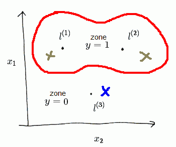
Say we have a $x$ near $l^{(1)}$ (green one on the left)
- we have $f^{(1)} \approx 1, f^{(2)} \approx 0, f^{(3)} \approx 0$
- putting it to the model we get
- $\theta_0 + \theta_1 f_1 + \theta_2 f_2 + \theta_3 f_3 \approx -0.5 + 1 = 0.5 \geqslant 0$
- so we predict $y = 1$
Next, say we have a $x$ close to $l^{(3)}$ (blue one on the bottom),
- so $f^{(1)} \approx 0, f^{(2)} \approx 0, f^{(3)} \approx 1$, and we have
- $\theta_0 + \theta_1 f_1 + \theta_2 f_2 + \theta_3 f_3 \approx -0.5 < 0 $
- so we predict $y = 0$
Thus in this example
- for points near $l^{(1)}$ and $l^{(2)}$ we end up predicting $y = 1$
- in other cases we predict $y = 0$
Choosing Landmarks
How to choose the landmarks?
- Suppose we have $m$ training examples ${(x^{(i)}, y^{(i)})}$
- Now we just put a landmark at the exactly same locations, i.e. l^{(i)} = x^{(i)}
- And we’ll end up with $m$ landmarks $l^{(i)}$
Usage Notes
- We need to perform Feature Scaling before applying Gaussian Kernel, or one feature may dominate over others.
Other Kernels
Mercer’s Theorem
- Not all similarity functions are valid kernels: they have to satisfy a condition called Mercer’s Theorem
- It makes sure they run correctly and don’t diverge (to support optimization)
Other kernels:
- No Kernel (or linear kernel)
- predict “$y = 1$” if $\theta^T x \geqslant 0$
- standard linear classifier
- Polynomial Kernel
- String Kernel
- Chi-square Kernel and so on
Training
- Given example $x^{(i)}$ we compute
- $f_1^{(i)} = \text{similarity}(x^{(i)}, l^{(1)})$
- $f_2^{(i)} = \text{similarity}(x^{(i)}, l^{(2)})$
- …
- $f_m^{(i)} = \text{similarity}(x^{(i)}, l^{(m)})$
- And we also add an extra feature $f_0 = 1$ (intercept term)
- That gives us a feature vector $f^{(i)} = [f_0^{(i)}, f_1^{(i)}, …, f_m^{(i)}]^T \in \mathbb{R}^{m + 1}$
- somewhere in this list we’ll have a feature $f_i^{(i)} = \text{similarity}(x^{(i)}, l^{(i)}) = 1$
Getting $\theta$
- To get $\theta$ we need to train our classifier
-
- recall that our objective function is
- $\min_{\theta} C \cdot \sum_{i = 1}^{m} \left [ y^{(i)} \cdot \text{cost}{1}(\theta^T x^{(i)}) + (1 - y^{(i)}) \cdot \text{cost}{0}(\theta^T x^{(i)}) \right] + \cfrac{1}{2} \sum_{j = 1}^{n} \theta_j^2$
- with Kernels, we now have $n = m + 1$ features
Let’s take a closer look at the second term
- as we know, this is an Inner Product:
-
$\sum_{j = 1}^{n} \theta_j^2 = | \theta |^2 = \theta^T \theta$ - In reality, for SVM implementation a re-scaled version is often used: - $\theta^T \cdot M \cdot \theta$
- which is a numerical optimization trick
Additional Notes
Hypothesis
Given $x$,
- compute features $f \in \mathbb{R}^{m + 1}$
- and predict $y = 1$ if $\theta^T f \geqslant 0$
- ($\theta$ also $\in \mathbb{R}^{m + 1}$)
SVM parameters
SVM has two parameters
- $C$ (which is equivalent to $\cfrac{1}{\lambda}$ where $\lambda$ is a Regularization term)
- large $C$: lower bias, higher variance (same as small $\lambda$): prone to overfitting
- small $C$: higher bias, lower variance (same as big $\lambda$): prone to underfitting
- $\sigma^2$ for Gaussian Kernels
- large $\sigma^2$: features $f_i$ vary more smoothly, results in higher bias, lower variance
- small $\sigma^2$: features $f_i$ vary less smoothly, results in lower bias, higher variance
see also Machine Learning Diagnosis
Multi-Class Classification
Use One-vs-All Classification:
- Train $K$ SVMs, each to distinguish $y = i$ from the rest
- Get $\theta^{(1)}, \theta^{(2)}, …, \theta^{(K)}$
- Pick class $i$ with largest $(\theta^{(i)})^T x$
SVN vs Other Classifiers
vs Logistic Regression
Suppose we have
- $n$ features ($x \in \mathbb{R}^{n + 1}$)
- $m$ training examples
if $n$ is large (relative to $m$)
- e.g. $n = 10000$, $m \in [10, 1000]$
- use Logistic Regression
- or SVM without kernel
if $n$ is small, $m$ in intermediate
- e.g. $n \in [1, 1000], m \in [10, 10000]$
- Use SVM with Gaussian Kernel
if $n$ is small, m is large
- say $n \in [1, 1000], m = 50000+ $
- SVM is too slow for that
- create more features
- then use Logistic Regression or SVM without a kernel
Logistic Regression and SVM without a kernel are pretty similar and have similar performance
vs Neural Networks
- Neural Networks are likely to work for all these cases, but they are slower to train.
- SVM models always have global optimum, whereas Neural Networks have local optima
See also
Links
- http://www.tristanfletcher.co.uk/SVM%20Explained.pdf