Decision Tree (Data Mining)

classifiers machine-learning

Decision Tree

This is a classification method used in Machine Learning and Data Mining that is based on Trees

not to confuse with Decision trees in Decision Analysis: Decision Tree (Decision Theory)

Rule-Based Classifiers

Suppose we have a set of rules

if we group them by condition
and then put redundant checks inside it
we get a decision tree

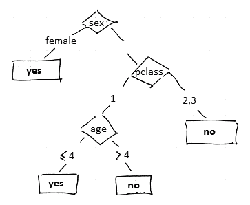
Rules:

IF pclass=’1’ AND sex=’female’ THEN survive=yes
IF pclass=’1’ AND sex=’male’ AND age < 5 THEN survive=yes
IF pclass=’2’ AND sex=’female’ THEN survive=yes
IF pclass=’2’ AND sex=’male’ THEN survive=no
IF pclass=’3’ AND sex=’male’ THEN survive=no
IF pclass=’3’ AND sex=’female’ AND age < 4 THEN survive=yes
IF pclass=’3’ AND sex=’female’ AND age >= 4 THEN survive=no

If we put if conditions inside

IF pclass=’1’ THEN
- IF sex=’female’ THEN survive=yes
- IF sex=’male’ AND age < 5 THEN survive=yes
IF pclass=’2’
- IF sex=’female’ THEN survive=yes
- IF sex=’male’ THEN survive=no
IF pclass=’3’
- IF sex=’male’ THEN survive=no
- IF sex=’female’
  - IF age < 4 THEN survive=yes
  - IF age >= 4 THEN survive=no

We have a decision tree:

Decision Trees

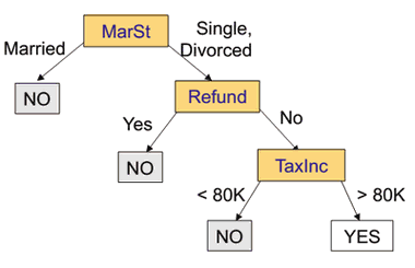
Consider this dataset

| Tid | Refund | Marital Status | Income | Cheat | 1 | Yes | Single | 125K | No || 2 | No | Married | 100K | No || 3 | No | Single | 70K | No || 4 | Yes | Married | 120K | No || 5 | No | Divorced | 95K | Yes || 6 | No | Married | 60K | No || 7 | Yes | Divorced | 220K | No || 8 | No | Single | 85K | Yes || 9 | No | Married | 75K | No || 10 | No | Single | 90K | Yes | There could be several decision trees for this dataset:

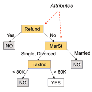
'’Decision Tree’’:

leaves are labels with the predicted class
internal nodes are labeled with attributes used to decide which path to take
edges are labeled with values for this attributes or with boolean tests

Classification:

suppose we take a previously unseen records (11, no, married, 112k, ?)
we need to predict a class for this label
we put this instance on top of the tree and go the way to the leaf
the leaf we end up is our class - cheat=no

Error Measures

A tree is ‘‘perfect’’ if it makes no errors on the training set

this tree is perfect w.r.t. the training dataset
learning error = 0%

Error measures:

learning error: # of errors on the training dataset
testing error: # of errors on the test set

Learning Algorithms

There are several learning algorithms

CART
ID3, C4.5
SLIQ, SPRINT, etc.

Main Principles

(ID3 algo)

Given:

training set $D$

The structure is recursive:

let $D_t$ be a set of records that reach a node $t$
at the beginning $t = \text{root}$ and $D_t \equiv D$
if all $d \in D_t$ belong to the same class $y_t$
- then $t$ is labeled by $y_t$
if $D_t \equiv \varnothing$
- then $t$ is labeled with the default class (e.g. the majority class)
if $d \in D_t$ belong to different classes
- split $D_t$ into subsets $D_{t+1}$ and recursively apply the procedure to each

Splitting

there is huge # of ways to split a set
how to determine the best split?

Splitting:

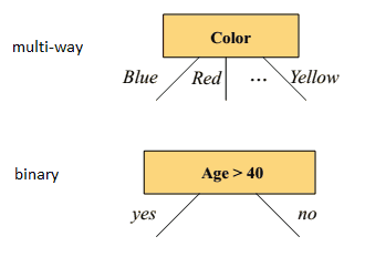
multiway: good for nominal, most of the time select all of the attributes
binary: good for numeric, but need to find where to split

Splitting numerical attributes

goal: want to find subsets that are more “pure” than the original one
“pure” = degree of homogeneity
$\fbox{$C_1$: 5, $C_2$: 5}$ - homogeneous, high degree of impurity
$\fbox{$C_1$: 9, $C_2$: 1}$ - non-homogeneous, low degree of impurity
the lower the better
use Information Gain for that

Stopping Conditions

Stop when

all records in node $k$ belong to the same class
the information gain is lower than some given threshold

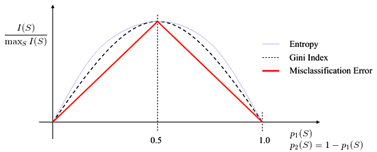
Information Gain

Given a set $S$ with $K$ classes $C_1, …, C_K$

let $p_k = \cfrac- $I(S)$ - is a function of impurity that we want to minimize

Measures of Impurity

Misclassification Error:
- $I(S) = 1 - \max_k p_k$
Entropy and Information Gain
- $I(S) = - \sum_k p_k \cdot \log_2 p_k$
Gini index:
- $I(S) = 1 - \sum_k p_k \cdot c_k$

Information Gain

how much information you get when partition the data?
def: $\Delta I = I(S) - p_L \cdot I(S_L) - p_R \cdot I(S_R)$
$p_L = \cfrac- $I$ - a measure of impurity

It’s easy to generalize IG to Multi-way

split $S$ to $K$ subsets $S_1, …, S_K$
$\Delta I = I(S) - \sum_k p_k \cdot I(S_k)$
$\sum_k p_k \cdot I(S_k)$ is the Expected Value of Entropy in the partitioned dataset
- $E \big[ I \big( { S_1, …, S_K } \big) \big] = \sum_k p_k I(S_k) = - \sum_k p_k \log_2 p_k$
- with $p_k = \cfrac- but if we minimize this $\Delta I$, we end up with $K = N$
- i.e. we obtain as many subsets as there are records - and a set with just one element is 100% pure
use Gain Ratio impurity
- $- \Delta I_K = \cfrac{\Delta I}{- \sum_k p_k \cdot \log_2 p_k}$

Example

Suppose we have a node with $S \equiv \fbox{$C_1$: 20, $C_2$: 30}$

$S_L \equiv \fbox{$C_1$: 15, $C_2$: 5}$ and $S_L \equiv \fbox{$C_1$: 5, $C_2$: 25}$
let $I$ be the Entropy function
$I(S) = - \cfrac{20}{50} \log_2 \cfrac{20}{50} - \cfrac{30}{50} \log_2 \cfrac{30}{50} \approx 0.971$
$I(S_L) = - \cfrac{15}{20} \log_2 \cfrac{15}{20} - \cfrac{5}{20} \log_2 \cfrac{5}{20} \approx 0.811$
$I(S_R) = - \cfrac{5}{30} \log_2 \cfrac{5}{30} - \cfrac{5}{30} \log_2 \cfrac{5}{30} \approx 0.65$
$\Delta I = I(S) - p_L \cdot I(S_L) - p_R \cdot I(S_R) = 0.971 - 0.4 \cdot 0.811 - 0.6 \cdot 0.65 = 0.26$

Another example with $S \equiv \fbox{$C_1$: 20, $C_2$: 30}$

suppose that now we want to split to $S_L \equiv \fbox{$C_1$: 10, $C_2$: 15}$ and $S_L \equiv \fbox{$C_1$: 10, $C_2$: 15}$
in this case it’s clear that we don’t have any IG
so min value is 0, and there’s no max boundary

Splitting Algorithm

for each attribute $A_i$

find the best partitioning $P^*_{A_i} = {S_1, …, S_K}$ of $S$
- $P^*_{A_i}$ maximizes the information gain
among all ${ P^*_{A_i} }$ select the maximal one
split by it

Best to split in halves: $K = 2$

how to choose $\alpha$ that splits $S$ into $S_L$ and $S_R$?
try several, pick up the best
note that $\Delta I$ is not monotonic - have to try all of them

Overfitting

Perfect decision trees perform 100% accurate on the training set

but perform very poorly on a test set
this is called Overfitting
when performing Machine Learning Diagnosis we see that the more nodes a decision tree has, the poorer it performs

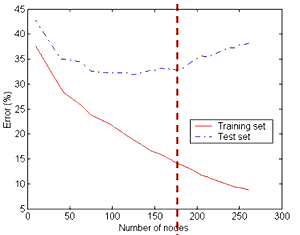
How to get the optimal complexity of a tree?

Pre-pruning
- Stop before a tree becomes perfect (fully-grown)
Post-pruning
- Grow a perfect tree
- Prune the nodes bottom-up

Pre-Pruning

It’s about finding a good stopping criterion

Simple ones:

when # of instances in a node goes below some threshold
when the misclassification error is lower than some threshold $\beta$
- $1 - \max_k p_k < \beta$
when expanding current node doesn’t give a significant information gain $\Delta I$
- $\Delta I < \beta$

More complex:

when class distribution of instances becomes independent from available features
- e.g. using Chi-square Test of Independence

Post-Pruning

Cost-Complexity Pruning

by Breiman, Olshen, Stone (1984)

Practical Issues

Decision Boundaries

the decision boundaries are rectilinear

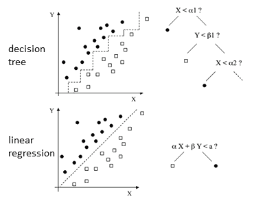
for some problems not always good
use another models: Linear Regression, Neural Networks etc

Handling Missing Values

Two options

discard all NAs
modify the algorithm

Algorithm Modification

Modification:

suppose that we have some splitting test criterion $T$ and dataset $S$
information gain for splitting $S$ using $T$ is
- $\Delta I (S, T) = I(S) - \sum_k \alpha_{T, k} \cdot I(S_k)$
let $S_0 \subseteq S$ for which we can’t evaluate $T$ (i.e. because needed values are missing)
if $S_0 \not \equiv \varnothing$
- calculate the information gain as
- $\cfrac- suppose such $T$ is chosen, what to do with values from $S_0$?
- add them to all the subsets with weight proportional to the size of these subsets
- $w_k = \cfrac - and information gain is computed using sums of weights instead of counts

Example

| X | Y | Z | Class | a | 70 | Yes | + || a | 90 | Yes | - || a | 85 | No | - || a | 95 | No | - || a | 70 | No | + || ? | 90 | Yes | + || b | 78 | No | + || b | 65 | Yes | + || b | 75 | No | + || c | 80 | Yes | - || c | 70 | Yes | - || c | 80 | No | + || c | 80 | No | + || c | 96 | No | + |

- There is one missing value for $X$: $(?, 90, \text{Yes}, +)$ - let $I$ be the misclassification error - $I(S - S_0) = 5/13$ (5 in "-", 8 in "+") - $I(S - S_0 | X = a) = 2/5$ |- $I(S - S_0 | X = b) = 0$ |- $I(S - S_0 | X = c) = 2/5$ |- calculate IG $\cfrac- $\Delta I = \cfrac{13}{14} \cdot (\cfrac{5}{13} - \cfrac{5}{13} \cdot \cfrac{2}{5} - \cfrac{3}{13} \cdot 0 - \cfrac{5}{13} \cdot \cfrac{2}{5}) = \cfrac{1}{14}$

Distribute the values to subsets

according to the value of $X$
but the rows with missing values are put to all the subsets
- and the weight is proportional to the size of this subset prior to adding these rows

| + $X = a$ || $Y$ | $Z$ | Class | $w$ || 70 | Yes | + | 1 || 90 | Yes | - | 1 || 85 | No | - | 1 || 95 | No | - | 1 || 70 | No | + | 1 || '''90''' | '''Yes''' | '''+''' | '''5/13''' |

| + $X = a$ || $Y$ | $Z$ | Class | $w$ || 78 | No | + | 1 || 65 | Yes | + | 1 || 75 | No | + | 1 || '''90''' | '''Yes''' | '''+''' | '''3/13''' |

| + $X = a$ || $Y$ | $Z$ | Class | $w$ || 80 | Yes | - | 1 || 70 | Yes | - | 1 || 80 | No | + | 1 || 80 | No | + | 1 || 96 | No | + | 1 || '''90''' | '''Yes''' | '''+''' | '''5/13''' |

Classification with Modification

Classification:

let $P(C E,T)$ be the probability of classifying case $E$ to class $C$ using tree $T$ - define it recursively:

if $t = \text{root}(T)$ is a leaf (i.e. it’s a singleton tree)

then P(C

E,T) is the relative frequency of training cases in class $C$ that reach $T$

- if $t = \text{root}(T)$ is not a leaf and $t$ is partitioned using attribute $X$

if $E.X = x_k$

then $P(C

E,T) = P(C

E,T_k)$ where $T_k$ is a subtree of $T$ where $X = x_k$

- if $E.X$ is unknown,

then $P(C

E,T) = \sum_{k=1}^{K} \cfrac - so we sum up probabilities of belonging to class $C$ from each child of $t$

- predict that a record belongs to class $C$ by selecting the highest probability $P(C

E,T)$

Example

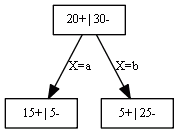
assume that $X$ is unknown - how to classify the case?

$P(+

E,T) = \sum_{k=1}^{K} P(+

E,T_k) = \cfrac{20}{50} \cdot \cfrac{15}{20} + \cfrac{30}{50} \cdot \cfrac{5}{30} = \cfrac{20}{50}$

- $P(-

E,T) = \sum_{k=1}^{K} P(-

E,T_k) = \cfrac{20}{50} \cdot \cfrac{5}{20} + \cfrac{30}{50} \cdot \cfrac{25}{30} = \cfrac{30}{50}$

- $P(-

E,T) > P(+

E,T) \Rightarrow$ predict “$-$”

Decision Tree Learning Examples

Example 1

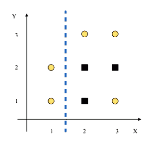
Suppose we have the following data:

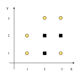
2 classes: $\square$ (S) and $\bigcirc$ (C)
there are 5S and 3C, total 8:
- $I(S) = - \frac{3}{8} \log_2 \frac{3}{8} - \frac{5}{8} \log_2 \frac{5}{8} = 0.954$
there are 2 attributes: $X$ and $Y$
- and 2 ways to split each: $X < 1.5, X < 2.5, Y < 1.5, Y < 2.5$

$S_L$

$I(S_L)$

$S_R$

$I(S_R)$

$E[I({S_L, S_R})]$

$\Delta I$

$X < 1.5$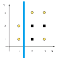

$2C$

$3C, 3S$

$\frac{2}{8} \cdot 0 + \frac{5}{8} \cdot 1 = 0.75$

$0.954 - 0.75 = \fbox{0.204}$

$X < 2.5$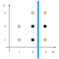

$3C, 2S$

0.971

$2C, 1S$

0.918

$\frac{5}{8} \cdot 0.971 + \frac{3}{8} \cdot 0.918 = 0.951$

0.003

$Y < 1.5$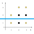

$2C, 1S$

0.918

$3C, 2S$

0.971

0.951

0.003

$Y < 2.5$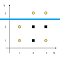

$2C$

$3C, 3S$

0.75

0.204

We decide to use $X < 1.5$ to split the data

left part is pure - no need to split it
right part: $3C, 3S$, it’s not pure: $I(S) = 1$

$I(S_L)$

$I(S_R)$

$\Delta I$

$X < 2.5$

0.918

0.082

$Y < 1.5$

$Y < 2.5$

0.811

$\fbox{0.459}$

$Y < 2.5$ - next best splitting criterion
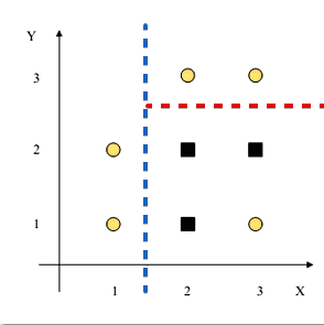
if we stop here, we obtain the following tree:
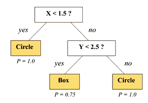
this tree is not a perfect tree - we can continue and at the end obtain a perfect one

Pros and Cons

Advantages

fast
handles both symbolic and numerical attributes
works well with redundant attributes
invariant to any monotonic transformation of the dataset
robust to Outliers
- e.g. a tree with $\text{income}$ will behave the same way as a tree with $\sqrt{\text{income}}$
easy to interpret and explain to non-specialists
help to understand what are most important attributes

Disadvantages

prone to overfitting, need pruning techniques
even a small variation in data can lead to very different tree
decision boundaries are rectilinear

Sources

✏️ Edit on GitHub